Regression analysis is crucial in predictive modeling, but merely running a line of code or looking at R² and MSE values isn’t enough. In R, the plot() function generates four plots that reveal valuable insights about the data. Unfortunately, many beginners fail to interpret these plots. This article explains important regression assumptions, fixes for violations, and the significance of these plots. Understanding these concepts can greatly enhance your regression models. Read on to learn all about the assumptions of linear regression and polynomial regression of these machine learning models.
All models are wrong, but some are useful
George Box
Table of contents
- What are Assumptions in Regression?
- What are Assumptions of Linear Regression?
- Important Assumptions of Linear Regression Analysis
- What Happens When You Violate the Assumptions of Linear Regression?
- Interpretation of Regression Plots
- How do you check the assumptions of linear regression before modeling?
- Conclusion
- Frequently Asked Questions
What are Assumptions in Regression?
Regression is a parametric approach. ‘Parametric’ means it makes assumptions about data for the purpose of analysis. Due to its parametric side, regression is restrictive in nature. It fails to deliver good results with data sets which doesn’t fulfill its assumptions. Therefore, for a successful regression analysis, it’s essential to validate these assumptions.
So, how would you check (validate) if a data set follows all regression assumptions? You check it using the regression plots (explained below) along with some statistical test.
What are Assumptions of Linear Regression?
Violations of assumptions of linear regression model can lead to biased or inefficient estimates, and it is important to assess and address these violations for accurate and reliable regression results.
6 Assumptions of linear regression include:
- Linearity: The relationship between the dependent and independent variables is linear.
- Independence: The observations are independent of each other.
- Homoscedasticity: The variance of the errors is constant across all levels of the independent variables.
- Normality: The errors follow a normal distribution.
- No multicollinearity: The independent variables are not highly correlated with each other.
- No endogeneity: There is no relationship between the errors and the independent variables.
Important Assumptions of Linear Regression Analysis
Let’s look at the important assumptions of Linear regression analysis:
- There should be a linear and additive relationship between dependent (response) variable and independent (predictor) variable(s). A linear relationship suggests that a change in response Y due to one unit change in X¹ is constant, regardless of the value of X¹. An additive relationship suggests that the effect of X¹ on Y is independent of other variables.
- There should be no correlation between the residual (error) terms. Absence of this phenomenon is known as Autocorrelation.
- The independent variables should not be correlated. Absence of this phenomenon is known as multicollinearity.
- The error terms must have constant variance. This phenomenon is known as homoskedasticity. The presence of non-constant variance is referred to heteroskedasticity.
- The error terms must be normally distributed.
What Happens When You Violate the Assumptions of Linear Regression?
Let’s dive into specific assumptions of linear regression and learn about their outcomes (if violated):
1. Linear and Additive
If you fit a linear model to a non-linear, non-additive data set, the regression algorithm would fail to capture the trend mathematically, thus resulting in an inefficient model. Also, this will result in erroneous predictions on an unseen data set.
How to check: Look for residual vs fitted value plots (explained below). Also, you can include polynomial terms (X, X², X³) in your model to capture the non-linear effect.
2. Autocorrelation
The presence of correlation in error terms drastically reduces model’s accuracy. This usually occurs in time series models where the next instant is dependent on previous instant. If the error terms are correlated, the estimated standard errors tend to underestimate the true standard error.
If this happens, it causes confidence intervals and prediction intervals to be narrower. Narrower confidence interval means that a 95% confidence interval would have lesser probability than 0.95 that it would contain the actual value of coefficients. Let’s understand narrow prediction intervals with an example:
For example, the least square coefficient of X¹ is 15.02 and its standard error is 2.08 (without autocorrelation). But in presence of autocorrelation, the standard error reduces to 1.20. As a result, the prediction interval narrows down to (13.82, 16.22) from (12.94, 17.10).
Also, lower standard errors would cause the associated p-values to be lower than actual. This will make us incorrectly conclude a parameter to be statistically significant.
How to check: Look for Durbin – Watson (DW) statistic. It must lie between 0 and 4. If DW = 2, implies no autocorrelation, 0 < DW < 2 implies positive autocorrelation while 2 < DW < 4 indicates negative autocorrelation. Also, you can see residual vs time plot and look for the seasonal or correlated pattern in residual values.
3. Multicollinearity
It occurs when the independent variables show moderate to high correlation. In a model with correlated variables, it becomes a tough task to figure out the true relationship of a predictors with response variable. In other words, it becomes difficult to find out which variable is actually contributing to predict the response variable.
Another point, with presence of correlated predictors, the standard errors tend to increase. And, with large standard errors, the confidence interval becomes wider leading to less precise estimates of slope parameters.
Additionally, when predictors are correlated, the estimated regression coefficient of a correlated variable depends on the presence of other predictors in the model. If this happens, you’ll end up with an incorrect conclusion that a variable strongly / weakly affects target variable. Since, even if you drop one correlated variable from the model, its estimated regression coefficients would change. That’s not good!
How to check: You can use scatter plot to visualize correlation effect among variables. Also, you can also use VIF factor. VIF value <= 4 suggests no multicollinearity whereas a value of >= 10 implies serious multicollinearity. Above all, a correlation table should also solve the purpose.
4. Heteroskedasticity
The presence of non-constant variance in the error terms results in heteroskedasticity. Generally, non-constant variance arises in presence of outliers or extreme leverage values. Look like, these values get too much weight, thereby disproportionately influences the model’s performance. When this phenomenon occurs, the confidence interval for out of sample prediction tends to be unrealistically wide or narrow.
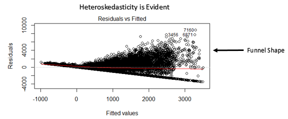
How to check: You can look at residual vs fitted values plot. If heteroskedasticity exists, the plot would exhibit a funnel shape pattern (shown in next section). Also, you can use Breusch-Pagan / Cook – Weisberg test or White general test to detect this phenomenon.
5. Normal Distribution of error terms
If the error terms are non- normally distributed, confidence intervals may become too wide or narrow. Once confidence interval becomes unstable, it leads to difficulty in estimating coefficients based on minimization of least squares. Presence of non – normal distribution suggests that there are a few unusual data points which must be studied closely to make a better model.
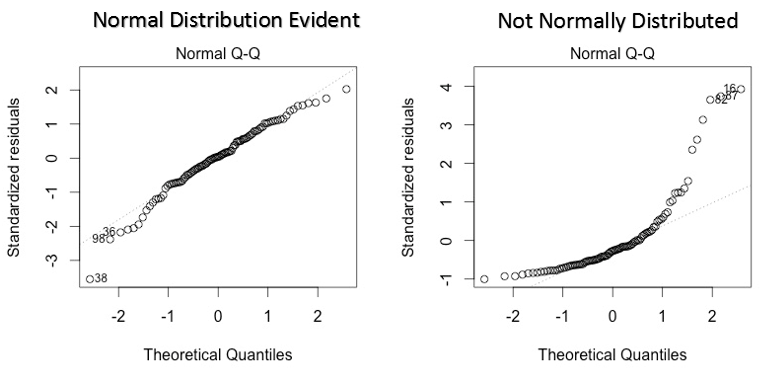
How to check: You can look at QQ plot (shown below). You can also perform statistical tests of normality such as Kolmogorov-Smirnov test, Shapiro-Wilk test.
Interpretation of Regression Plots
Now, we know all about important assumptions of linear regression and the methods take care of them in case of violation.
But that’s not the end. Now, you should know the solutions also to tackle the violation of these assumptions. In this section, I’ve explained the 4 regression plots along with the methods to overcome limitations on assumptions.
1. Residual vs Fitted Values


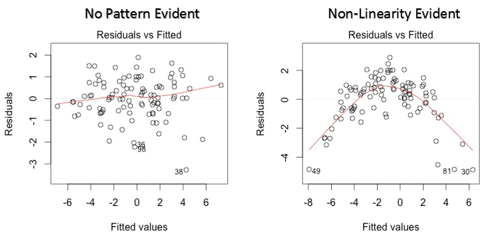
This scatter plot shows the distribution of residuals (errors) vs fitted values (predicted values). It is one of the most important plot which everyone must learn. It reveals various useful insights including outliers. The outliers in this plot are labeled by their observation number which make them easy to detect.
There are two major things which you should learn:
- If there exist any pattern (may be, a parabolic shape) in this plot, consider it as signs of non-linearity in the data. It means that the model doesn’t capture non-linear effects.
- If a funnel shape is evident in the plot, consider it as the signs of non constant variance i.e. heteroskedasticity.
Solution: To overcome the issue of non-linearity, you can do a non linear transformation of predictors such as log (X), √X or X² transform the dependent variable. To overcome heteroskedasticity, a possible way is to transform the response variable such as log(Y) or √Y. Also, you can use weighted least square method to tackle heteroskedasticity.
2. Normal Q-Q Plot

This q-q or quantile-quantile is a scatter plot which helps us validate the assumption of normal distribution in a data set. Using this plot we can infer if the data comes from a normal distribution. If yes, the plot would show fairly straight line. The straight lines shows the absence of normality in the errors.
If you are wondering what is a ‘quantile’, here’s a simple definition: Think of quantiles as points in your data below which a certain proportion of data falls. Quantile is often referred to as percentiles. For example: when we say the value of 50th percentile is 120, it means half of the data lies below 120.
Solution: If the errors are not normally distributed, non – linear transformation of the variables (response or predictors) can bring improvement in the model.
3. Scale Location Plot

This plot is also detects homoskedasticity (assumption of equal variance). It shows how the residual are spread along the range of predictors. It’s similar to residual vs fitted value plot except it uses standardized residual values. Ideally, there should be no discernible pattern in the plot. This would imply that errors are normally distributed. But, in case, if the plot shows any discernible pattern (probably a funnel shape), it would imply non-normal distribution of errors.
Solution: Follow the solution for heteroskedasticity given in plot 1.
4. Residuals vs Leverage Plot

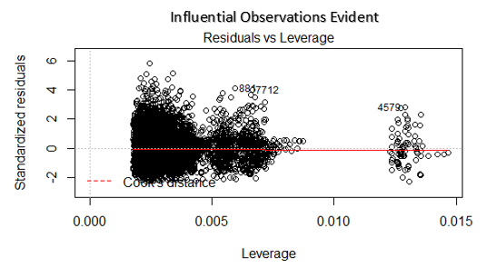
Cook’s distance attempts to identify the points which have more influence than other points. Such influential points tends to have a sizable impact of the regression line. In other words, adding or removing such points from the model can completely change the model statistics.
But, can these influential observations be treated as outliers? Only data can answer this question.. Therefore, in this plot, the large values marked by cook’s distance might require further investigation.
Solution: For influential observations which are nothing but outliers, if not many, you can remove those rows. Alternatively, you can scale down the outlier observation with maximum value in data or else treat those values as missing values.
Case Study: How I improved my regression model using log transformation
How do you check the assumptions of linear regression before modeling?
Here is you can check the Assumptions of linear regression
- Linearity: This denotes a nearly straight line-like relationship between the independent and dependent variables in a multiple linear regression. Plotting your data in a scatter plot will help you see this. Look for a haphazard dispersion surrounding a line segment, which suggests that the linearity assumption is met.
- Independence: The inaccuracies, or variations between the expected and actual values, ought to be unrelated to one another. This indicates that no error term affects another, which is crucial when dealing with time series data. Plotting the residuals, or errors, against the independent variables allows you to evaluate this. Ideally, there should be no trends or patterns.
- Homoscedasticity: For every level of the independent variables, the variance of the errors should remain constant. In other words, the distribution of residuals should be consistent across the entire range of the independent variables. To check for heteroscedasticity, make a residual vs. fitted plot. The red line, representing the fitted values, should ideally have a horizontal line centered around zero.
- Normality: A normal distribution should be present in the errors (residuals). You can verify this by using Q-Q plots of the residuals or histograms. Additionally, statistical tests such as the Kolmogorov-Smirnov test can be used to check the normality assumption.
- Lack of Multicollinearity: There should be little to no significant correlation between the independent variables. Multicollinearity can make it difficult to interpret your model’s coefficients. Correlation matrices (preferably with correlation coefficients less than 0.8) or the Variance Inflation Factor (VIF) can be used to test for this. Values greater than or equal to 10 indicate significant multicollinearity.
Conclusion
In conclusion, understanding and acknowledging the assumptions of linear regression is vital for accurate and reliable analysis. By recognizing the regression assumptions, we can ensure the validity of our models and interpret the results effectively. It is essential to assess the assumptions and address any violations to enhance the reliability of our findings. Adhering to these assumptions allows us to make informed decisions and draw meaningful insights from assumptions of linear regression analyses in various data science applications.
Frequently Asked Questions
A. The assumptions of linear regression in data science are linearity, independence, homoscedasticity, normality, no multicollinearity, and no endogeneity, ensuring valid and reliable regression results.
A. Regression analysis relies on the assumptions of linearity, independence, homoscedasticity, and normality to interpret and validate the model.
Linearity: The relationship between variables is linear.
Independence: Observations are independent of each other.
Homoscedasticity: The variance of the errors is constant.
Normality of Residuals: Residuals follow a normal distribution.
No Multicollinearity: Predictor variables are not highly correlated.
A. The assumptions of regression error include independence, zero mean, constant variance, and normality, ensuring adherence to the regression model’s assumptions.


Thanks for the really nice article. this part of regression is mostly missed by many.
Glad you found it helpful. I've seen regression algorithm shows drastic model improvements when used with techniques I described above. I hope it help others as well.
Small edit: Durbin Watson d values always lie between 0 and 4. A value of d=2 indicates no autocorrelation. A value between 0-2 indicates positive correlation while a value between 2-4 indicates negative correlation. Please correct the blog.
Thanks Vivek. I just checked and found that's correct. Made the changes.
This is a good article. I have a comment on the Residuals vs Leverage Plot and the comment about it being a Cook's distance plot. Although you mention this as a Cook's distance plot, and mark Cook's distance at std residual of -2, this seems incorrect. It looks like you have plotted standardized residuals e=(I-H)y vs leverage (hii from hat matrix H). And the +/- 2 cutoff is typically from R-student residuals. If you had plotted Cook's distance, the cutoff would typically be 1 or 4/n. Correct me if I'm wrong here, thanks!
Hi Rahul, I think the marked cook's distance at -2 is just a legend which shows cook's distance can be determined by the red dotted line. After creating, residual vs leverage plots based on other data sets, I came to this conclusion.
I find the article useful especially for guys planning to join data analytic field. However, I find this number two and three confusing There should be no correlation between the residual (error) terms. Absence of this phenomenon is known as Autocorrelation. The independent variables should not be correlated. Absence of this phenomenon is known as multicollinearity.
The stages of modeling are Identification, Estimation,Diagnostic checking and then Forecasting as laid out by Box-Jenkins in their 1970 text book "Time Series Analysis: Forecasting and Control". The idea is to identify if there is relationship using the cross-correlation function instead of assuming one. In fact, there might be MSB (model specification bias)if you assume. There might be a lead or lag relationship to complicate matters. A bivariate normalized scatter plot is also very helpful. The one item that no one ever covers (except us) is looking for outliers and changes with multivariate data(change in trend, level, seasonality,parameters,variance). If you aren't looking for these then you just skipped "diagnostic checking" so that your residuals are random with constant mean and variance. Try this example and see how you do....http://bit.ly/29kLC1g Good luck!
Thanks for the writeup.. How can we identify which predictors from a large set of predictors have a non-linear impact on the model?
Regarding the first assumption of regression;"Linearity"-the linearity in this assumption mainly points the model to be linear in terms of parameters instead of being linear in variables and considering the former, if the independent variables are in the form X^2,log(X) or X^3;this in no way violates the linearity assumption of the model. Then how can I use these polynomial terms to correct non linearity, when there presence, with linear parametrs is maintaining the model's linearity assumption.
All your contributions are very useful for professionals and non professionals. I appreciate your availability to share the must know issues to get better society.
when considering the linearity assumption, are you considering the model to be linear in variables only or linear in parameters only?
Hi Manish, Can You Plz suggest the the best book to study Data analysis so deep as you explained in your article. I want to study root concepts so that my thinking ability enhances . Thanks a million. Ramit Pandey
Hi Ramit, If you want to learn from scratch, you can read Introduction to Statistical Learning. It's freely available in PDF version.
Hi Manish , Could you please explain the scaling of these graphs ? what does -2 , -4 , 4 , 6, 8 represent on X axis and Y axis ? Thanks, Ankur
Really good article. Thank you so much. Could you please give us some explanation about logistic regression with these plots?
Same with Jack. Could you please share an article about Logistic Regression analysis? Thank you so much!!!
I would like to differ on the assumptions of linear regression. Linear regression does not make any direct assumption about the zero auto-correlation of the error terms. It does assume that the observations are randomly selected after the assumption of linearity and additive phenomena. Also the last assumption of normality of error terms is relaxed when a sufficiently large sample of data is present.
Awesome job mate with the plots, assumptions and explanation ... A few tests for normality i never heard of .... Please do one for logistic regression also XD
Wow cuz this is very helpfulexcellent work! Congrats and keep it up
It really helps when these topics are broken down in an intuitive and consumable way. And you did it very well! Can't wait to read more...
Can you explain heteroskedasticiy more in detail .I am not able to understand it properly.Is it always the funnel which defines heteroskedasticiy in the model.
Comments are Closed