With the evolution of neural networks, various tasks which were considered unimaginable can be done conveniently now. Tasks such as image recognition, speech recognition, finding deeper relations in a data set have become much easier. A sincere thanks to the eminent researchers in this field whose discoveries and findings have helped us leverage the true power of neural networks.
If you are truly interested in pursuing machine learning as a subject, a thorough understand of deep learning networks is crucial for you. Most ML algorithms tend of lose accuracy when given a data set with several variables, whereas a deep learning model does wonders in such situations.. Therefore, it’s important for us to understand how does it work!
In this article, I’ve explained the core concepts used in deep learning i.e. what sort of backend calculations result in enhanced model accuracy. Along side, I’ve also shared various modeling tips and a sneak peek into the history of neural networks.
Overview of Deep Learning
About The Authors
Neural networks are the building blocks of today’s technological breakthrough in the field of Deep Learning. A neural network can be seen as simple processing unit that is massively parallel, capable to store knowledge and apply this knowledge to make predictions.
A neural network mimics the brain in a way the network acquires knowledge from its environment through a learning process. Then, intervention connection strengths known as synaptic weights are used to store the acquired knowledge. In the learning process, the synaptic weights of the network are modified in an orderly fashion to attain the desired objective. In 1950, the neuro-psychologist Karl Lashley’s thesis was published in which he described the brain as a distributed system.
Another reason that the neural network is compared with the human brain is that, they operate like non-linear parallel information-processing systems which rapidly perform computations such as pattern recognition and perception. As a result, these networks perform very well in areas like speech, audio and image recognition where the inputs / signals are inherently nonlinear.
McCulloch and Pitts were pioneers of neural networks who wrote a research article on the model with two inputs and single output in 1943. The following were the features of that model:
A neuron would only be activated if:
There is a certain threshold level computed by summing up the input values for which the output is either zero or one.
In Hebb’s 1949 book ‘The Organization of Behaviour’, the idea that the connectivity of brain is continuously changing in response to changes in tasks was proposed for the first time. This rule implies that the connection between two neurons is active at the same time. This soon became the source of inspiration for the development of computational models of learning and adaptive systems.
Artificial neural networks have the ability to learn from supplied data, known as adaptive learning, while the ability of a neural network to create its own organization or representation of information is known as self-organisation.
After 15 years, the perceptron developed by Rosenblatt in 1958 emerged as the next model of neuron. Perceptron is the simplest neural network that linearly separates the data into two classes. Later, he randomly interconnected the perceptron and used a trial and error method to change the weights for the learning.
After 1969, the research came to a dead end in this area for the next 15 years after the mathematicians Marvin Minsky and Seymour Parpert published a mathematical analysis of the perceptron. They found that the perceptron was not capable of representing many important problems, like the exclusive-or function (XOR). Secondly, there was an issue that the computers did not have enough processing power to effectively handle large neural networks.
In 1986, the development of the back-propagation algorithm was reported by Rumelhart, Hinton, and Williams that can solve problems like XOR, beginning a second generation of neural networks. In that same year, the celebrated two-volume book, Parallel Distributed Processing: Explorations in the Microstructures of Cognition, edited by Rumelhart and McClelland, was published. That book has been a major influence in the use of back-propagation, which has emerged as the most popular learning algorithm for the training of multilayer perceptrons.
The simplest type of perceptron has a single layer of weights connecting the inputs and output. In this way, it can be considered the simplest kind of feed-forward network. In a feed forward network, the information always moves in one direction; it never goes backwards.
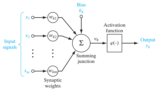
Figure 1
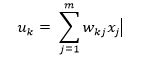
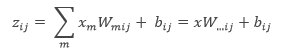
Figure 1 shows a single-layer perceptron for easier conceptual grounding and clarification into multilayer perceptron (explained ahead). Single layer perceptron represents the m weights that are seen as a set of synapses or connecting links between one layer and another layer within the network. This parameter indicates how important each feature ![]() is. Below is the adder function of features of the input multiplied by their respective synaptic connection:
is. Below is the adder function of features of the input multiplied by their respective synaptic connection:
The bias ![]() , acts as an affine transformation to the output of the adder function
, acts as an affine transformation to the output of the adder function ![]() giving
giving ![]() , the induced local field as:
, the induced local field as:
![]()
Moving onwards, multi-layer perceptron, also known as feed-forward neural networks, consists of a sequence of layers each fully connected to the next one.
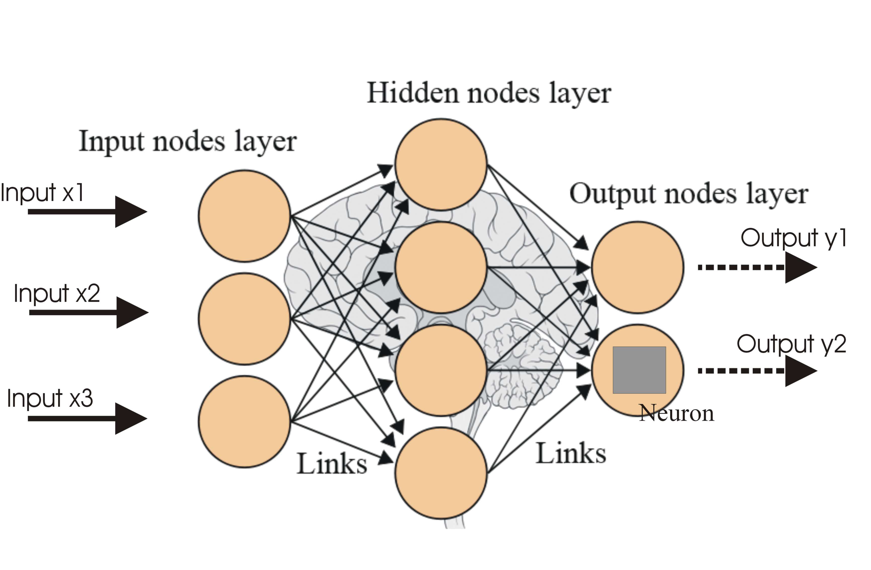
A multilayer perceptron (MLP) has one or more hidden layers along with the input and output layers, each layer contains several neurons that interconnect with each other by weight links. The number of neurons in the input layer will be the number of attributes in the dataset, neurons in the output layer will be the number of classes given in the dataset.
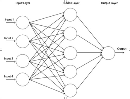 Figure 2
Figure 2 shows a multilayer perceptron where we have three layers at least and each layer is connected to the last one. To make the architecture deep, we need to introduce multiple hidden layers.
Initialization of the parameters, weights and biases plays an important role in determining the final model. There is a lot of literature on initialization strategy.
A good random initialization strategy can avoid getting stuck at local minima. Local minima problem is when the network gets stuck in the error surface and does not go down while training even when there is capacity left for learning.
Doing experiment by using various initialization strategies is out of the scope of this research work.
The initialization strategy should be selected according to the activation function used. For tanh the initialization interval should be ![]() where
where ![]() is the number of units in the (i-1)-th layer, and
is the number of units in the (i-1)-th layer, and ![]() is the number of units in the ith layer. Similarly for the sigmoid activation function the initialization interval should be
is the number of units in the ith layer. Similarly for the sigmoid activation function the initialization interval should be ![]() . These initialization strategies ensure that information propagated upwards and backwards in the network at the early stage of training.
. These initialization strategies ensure that information propagated upwards and backwards in the network at the early stage of training.
The activation function defines the output of a neuron in terms of the induced local field v as:
![]()
where φ(.) is the activation function. There are various types of activation functions, the following are the commonly used ones:
![]()
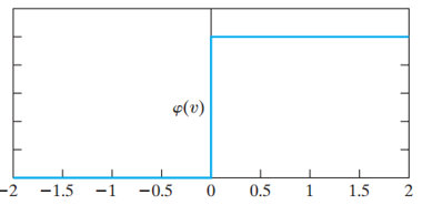
Figure 2
Figure 2 indicates that either the neuron is fully active or not. However, this function is not differentiable which is quite vital when using the back-propagation algorithm (explained later).
The sigmoid function is a logistic function bounded by 0 and 1, as with the threshold function, but this activation function is continuous and differentiable.
![]()
where α is the slope parameter of the above function. Moreover, it is nonlinear in nature that helps to increase the performance making sure that small changes in the weights and bias causes small changes in the output of the neuron.
φ (v) = tanh (v)
This function enables activation functions to range from -1 to +1.
ReLUs are the smooth approximation to the the sum of many logistic units and produce sparse activity vectors. Below is the equation of the function: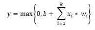
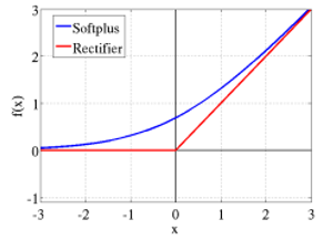
Figure 3
In figure 3, ![]() is the smooth approximation to the rectifier).
is the smooth approximation to the rectifier).
In 2013, Goodfellow found out that the Maxout network using a new activation function is a natural companion to dropout.
Maxout units facilitate optimization by dropout and improve the accuracy of dropout’s fast approximate model averaging technique. A single maxout unit can be interpreted as making a piece wise linear approximation to an arbitrary convex function.
Maxout networks learn not just the relationship between hidden units, but also the activation function of each hidden unit. Below is the graphical depiction of how this works:
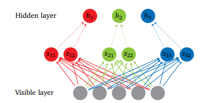
Figure 4
Figure 4 shows the Maxout network with 5 visible units, 3 hidden units and 2 pieces for each hidden unit.
![]()
where ![]() is the mean vector of size of the input obtained by accessing the matrix W ∈
is the mean vector of size of the input obtained by accessing the matrix W ∈ ![]() at the second coordinate i and third coordinate j . The number of intermediate units ( k ) is called the number of pieces used by the Maxout nets.
at the second coordinate i and third coordinate j . The number of intermediate units ( k ) is called the number of pieces used by the Maxout nets.
The back-propagation algorithm can be used to train feed forward neural networks or multilayer perceptrons. It is a method to minimize the cost function by changing weights and biases in the network. To learn and make better predictions, a number of epochs (training cycles) are executed where the error determined by the cost function is backward propagated by gradient descent until a sufficiently small error is achieved.
Let’s say in 100-sized mini-batch, 100 training examples are shown to the learning algorithm and weights are updated accordingly. After all mini-batches are presented sequentially, the average of accuracy levels and training cost levels are calculated for each epoch.
Stochastic gradient descent is used in the real-time on-line processing, where the parameters are updated while presenting only one training example, and so average of accuracy levels and training costs are taken for the entire training dataset at each epoch.
In this method all the training examples are shown to the learning algorithm and the weights are updated.
There are various cost functions. Below are some examples:
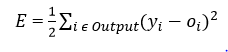
where ![]() is the predicted output
is the predicted output ![]() is the actual output
is the actual output
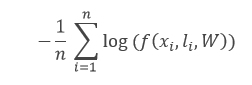
where the f function is the model’s predicted probability for the input ![]() label to be
label to be ![]() , W are its parameters, and n is the training-batch size.
, W are its parameters, and n is the training-batch size.
NLL is the cost function used in all the experiments of the report.
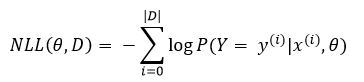
where ![]() is the value of the output is,
is the value of the output is, ![]() is the value of the feature input, θ is the parameters and D is the training set.
is the value of the feature input, θ is the parameters and D is the training set.
Learning rate controls the change in the weight from one iteration to another. As a general rule, smaller learning rates are considered as stable but cause slower learning. On the other hand higher learning rates can be unstable causing oscillations and numerical errors but speed up the learning.
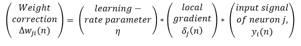
Momentum provides inertia to escape local minima; the idea is to simply add a certain fraction of the previous weight update to the current one, helping to avoid becoming stuck in local minima.
![]()
where α is the momentum.
Softmax is a neural transfer function that is generalized form of logistic function implemented in the output layer that turns the vectors into the probabilities that add up and constraint to 1.
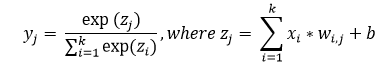
For classification, a softmax function may be incorporated in the output layer that will give the probability of each occurring class. Activation function is used to compute the predicted output of each neuron in each layer by using inputs, weights and bias.
The back propagation method trains the multilayer neural network by modifying its synaptic connection weights between the layers to improve model performance based on the error correction learning function which needs to be continuous and differentiable. The following parameters have been evaluated in the experiments:
Before 2006, various failed attempts at training deep supervised feed forward neural networks were made that resulted in over-fitting of the performance on the unseen data i.e. training error reduces while validation error increases.
A deep network usually means an artificial neural network that has more than one hidden layer. Training the deep hidden layers required more computational power. Having a greater depth seemed to be better because intuitively neurons can make the use of the work done by the neuron in the layer below resulting in distributed representation of the data.
Bengio suggests that the neurons in the hidden layers are seen as feature detectors learned by the neuron in the below layer. This result in better generalization that is a subset of neurons learns from data in a specific region of the input space.
Moreover deeper architectures can be more efficient as fewer computational units are needed to represent the same functions, achieving greater efficiency. The core idea behind the distributed representation is the sharing of statistical strengths where different components of the architecture are re-used for different purposes.
Deep neural architectures are composed of multiple layers utilizing non-linear operations, such as in neural nets with many hidden layers. There are often various factors of variation in the dataset, like aspects of the data separately and often independently may vary.
Deep Learning algorithms can capture these factors that explain the statistical variations in the data, and how they interact to generate the kind of data we observe. Lower level abstractions are more directly tied to particular observations; on the other hand higher level ones are more abstract because their connection to perceived data is more remote.
The focus of deep architecture learning is to automatically discover such abstractions, from low level features to the higher level concepts. It is desirable for the learning algorithms to enable this discovery without manually defining necessary abstractions.
Training samples in the dataset must be at least as numerous as the variations in the test set otherwise the learning algorithm cannot generalize. Deep Learning methods aim to learn feature hierarchies, composing lower level features into higher level abstractions.
Deep neural nets with a huge number of parameters are very powerful machine learning systems. However, over-fitting is a serious problem in deep networks. Over-fitting is when the validation error starts to go up while the training error declines. Dropout is one of the regularization techniques for addressing this problem which is discussed later.
Today one of the most important factors for the increased success of Deep Learning techniques is advancement in the computing power. Graphical Processing Units (GPU) and cloud computing are crucial for applying Deep Learning to many problems.
Cloud computing allows clustering of computers and on demand processing that helps to reduce the computation time by paralleling the training of the neural network. GPU’s, on the other hand, are special purpose chips for high performance mathematical calculations, speeding up the computation of matrices.
In 2006-07, three papers revolutionized the deep learning discipline. The key principles in their work were that each layer can be pre-trained by unsupervised learning, done one layer at a time. Finally supervised training by back-propagation of the error is used to fine-tune all the layers, effectively giving better initialization by unsupervised learning than by random initialization.
One of the unsupervised algorithms is Restricted Boltzmann Machines (RBM) that is used to pre-train deep belief network. The RBM is a simplified version of the Boltzmann Machine, inspired by statistical mechanics, which models energy based probabilities for the underlying distributions of the given data sets from which conditional distributions can be derived.
Boltzmann Machines are bidirectionally connected networks of stochastic processing units of visible units and hidden units. The raw data corresponds to the ‘visible’ neurons and samples to observed states and the feature detectors correspond to ‘hidden’ neurons. In a Boltzmann Machine, visible neurons provide the input to the network and the environment in which it operates. During training visible neurons are clamped (set to a defined value) determined by the training data. Hidden neurons on the other hand operate freely.
However, Boltzmann Machine are difficult to train because of its connectivity. An RBM has restricted connectivity to make learning easier; there are no connections between hidden units in a single layer forming a bipartite graph, depicted in figure 2. The advantage of this is that the hidden units are updated independently and in parallel given the visible state.
These networks are governed by an energy function that determines the probability of the hidden/visible states. Each possible joint configuration of the visible and hidden units has a Hopfield energy determined by the weights and biases. The energies of the joint configurations are optimized by Gibbs sampling that learns the parameters by minimizing the lowest energy function of the RBM.
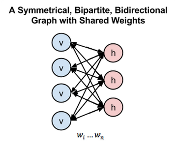
Figure 5
In figure 5, left layer represents the visible layer and right layer represents the hidden layer.
In Deep Belief Network (DBN), RBM is trained by input data with important features of the input data captured by stochastic neurons in the hidden layer. In the second layer the activations of the trained features are treated as input data. The learning process in the second RBM layer can be viewed as learning feature of features. Every time a new layer of features is added to the deep belief network, a variational lower bound on the log-probability of the original training data is improved.
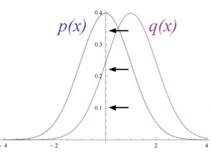
Figure 6
Figure 6 shows RBM converts its data distribution into a posterior distribution over its hidden units.
The weights of the RBM are randomly initialized causing the difference in the distribution of p(x) and q(x). During learning, weights are iteratively adjusted to minimize the error between p(x) and q(x). In figure 2 q(x) is the approximate of the original data and p(x) is the original data.
The rule for adjusting the synaptic weight from neuron one and another is independent of whether both the neurons are visible or hidden or one of each. The updated parameters by the layers of RBM are used as initialization in DBN’s that fine-tunes all the layers by supervised training of backpropagation.
For the IDS data of KDD Cup 1999, it is appropriate to use multimodal (Bernoulli-Gaussian) RBM as KDD Cup 1999 consists of mixed data types, specifically continuous and categorical. In multimodal RBM there are two different channel input layers used in the RBM, one is Gaussian input unit used for continuous features and the other one is Bernoulli input unit layer where binary features are used. Using multimodal RBM is beyond the scope of this research work.
Recent developments have introduced powerful regularizers to deep networks to reduce over-fitting. In machine learning, regularization is additional information usually introduced in the form of a penalty to penalize complexity of the model that leads to over-fitting.
Dropout is a regularization technique for deep neural networks introduced by Hinton which consists of preventing co-adaptation of feature detectors by randomly turning off a portion of neurons at every training iteration but using the entire network (with weights scaled down) at test time.
Dropout reduces over-fitting by being equivalent to training an exponential number of models that share weights. There exists an exponential number of different dropout configurations for a given training iteration, so a different model is almost certainly trained every time. At test time, the average of all models is used, which acts as a powerful ensemble method.
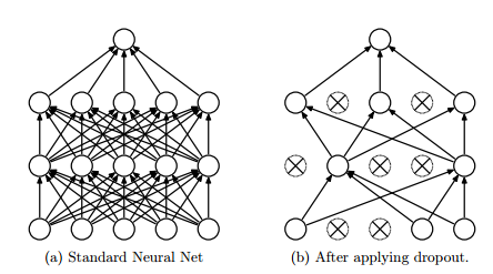
Figure 7
In figure 7, dropout randomly drops the connections between the neural network layer
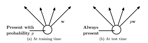
Figure 8
In figure 8, at training time the connections are dropped with probability, while at the test time weights are scaled to ρw
Averaging many models usually has been the key for many winner of the machine learning competitions. Many different types of model are used and then combined to make predictions at test time.
Random forest is a very powerful bagging algorithm which is created by averaging many decision trees giving them different training sample sets with replacement. It is well known that the decision trees are easy to fit to data and fast at test time so averaging different individual trees by giving them different training sets is affordable.
However, using the same approach with deep neural networks will prove to be very computationally expensive. It is already costly to train individual deep neural networks and training multiple deep neural networks and then averaging seems to be impractical. Moreover a single network that is efficient at test time is needed rather than having lots of large neural nets.
Dropout is an efficient way to average many large neural nets. Each time while training the model hidden units can be omitted with some probability as in figure 8, which is usually ρ= 0.5, when the training example is presented. As a result a ‘mean network’ model that has all the outgoing weights halved is used at test time as in figure 4. The mean network is equivalent to taking the geometric mean of the probability distributions over labels predicted by all possible networks with a single hidden layer of units and ‘softmax’ output layer.
As per the is mathematical proof of how dropout can be seen as an ensemble method.
![]() is the prediction of the “ensemble” using the geometric mean.
is the prediction of the “ensemble” using the geometric mean.
![]() is the prediction of a single sub model.
is the prediction of a single sub model.
d is the binary vector that tells which inputs to include into the softmax classifier.
![]()
Suppose there are different units. There will be 2^N possible assignments to d, and so;
![]() where y is the single and
where y is the single and ![]() is the vector of the classes index.
is the vector of the classes index.
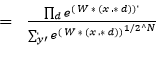
The sum of the probabilities of the output by a single sub-model is used to normalize ![]()
![]()
![]() , as per the definition of softmax
, as per the definition of softmax
![]()
![]()
![]()
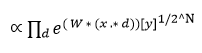
So, the predicted probability must be proportional to this. To re-normalize the above expression, it is divided by ![]() which means the predicted probability distribution is
which means the predicted probability distribution is ![]()
Another way to view dropout is that, it is able to prevent co-adaption among the feature detectors. Co-adaption of the feature detector means that if a hidden unit knows which other hidden units are present, it can co-adapt with them on the training data. However, on the test dataset complex co-adaptions are likely to fail to generalize.
Dropout can also be used in the input layer at a lower rate, typically 20% probability. The concept here is the same as de-noising auto encoders developed. In this method some of the inputs are omitted. This hurts the training accuracy but improves generalization acting in a similar way as adding noise to the dataset while training.
In 2013 a variant of dropout is introduced called Drop connect. Instead of dropping hidden units with certain probability weights are randomly dropped with certain probability. It has been shown that a Drop connect network seemed to perform better than dropout on the MNIST data set.
A class imbalance problem arises when one of the classes (minority class) is heavily under-represented in comparison to the other classes (majority class). This problem has real world significance where it is costly to misclassify minority classes such as detecting anomalous activities like fraud or intrusion. There are various techniques to deal with the class imbalance problem such as explained below:
One widely used approach to address the class imbalance problem is resampling of the data set. The sampling method involves pre-processing and balances the training data set by adjusting the prior distribution for minority and majority classes. SMOTE is an over-sampling approach in which the minority class is over-sampled by creating “synthetic” examples rather than by over-sampling with replacement.
It has been suggested that oversampling the minority class by replacement does not improve the results significantly rather it tends to over-fit the classification of the minority class. Instead the SMOTE algorithm operates in ‘feature space’ rather than ‘data space’. It creates synthetic samples by oversampling the minority class which tends to generalize better.
The idea is inspired by creating extra training data by operating on real data so that there is more data that helps to generalize prediction.
In this algorithm firstly nearest neighbours are computed for the minority class. Then, synthetic samples of the minority class are computed in the following manner: a random number of nearest neighbours is chosen and distance between that neighbour and the original minority class data point is taken.
This distance is multiplied by a random number between 0 and 1 and adds the result to the feature vector of the original minority class data as an additional sample, thus creating synthetic minority class samples.
Cost sensitivity learning seems to be quite an effective way to address the class imbalance for classification problems. Three cost sensitive methods have been described that are specific to neural networks.
Incorporate the prior probabilities of the class in the output layer of the neural network while testing unseen examples
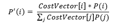
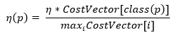
Adjusted learning rates based on the costs. Higher learning rates should be assigned to examples with high misclassifications costs making a larger impact on the weight changes for those examples
Modifying the mean square error function. As a result, the learning done by backpropagation will minimize misclassification costs. The new error function is:
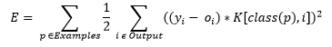
with the cost factor being K[i,j].
This new error function results in a new delta rule used in the updating of the weights of the network: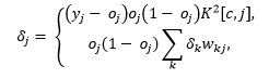
where the first equation represents the error function for output neurons and the second equation represents the error function for hidden neurons.
If you are not comfortable with math, the mathematical functions explained above might seem intimidating to you. Therefore, you are advised to undergo online courses on algebra and integrals.
In this article, we discussed the core concepts of deep learning such as gradient descent, backpropagation algorithm, cost function etc and their respective role in building a robust deep learning model. This article is a result of our research work done on deep learning. Hope you found this article helpful. And to gain expertise in working in neural network try out the deep learning practice problem – Identify the Digits.
Have you done any research of a similar topics ? Let us know your suggestions / opinions on building powerful deep learning models.
Lorem ipsum dolor sit amet, consectetur adipiscing elit,


Clearly explained ...