24 minutes
Before we start, have a look at the below examples.
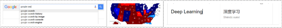
So what do the above examples have in common?
You possible guessed it right – TEXT processing. All the above three scenarios deal with humongous amount of text to perform different range of tasks like clustering in the google search example, classification in the second and Machine Translation in the third.
Humans can deal with text format quite intuitively but provided we have millions of documents being generated in a single day, we cannot have humans performing the above the three tasks. It is neither scalable nor effective.

So, how do we make computers of today perform clustering, classification etc on a text data since we know that they are generally inefficient at handling and processing strings or texts for any fruitful outputs?
Sure, a computer can match two strings and tell you whether they are same or not. But how do we make computers tell you about football or Ronaldo when you search for Messi? How do you make a computer understand that “Apple” in “Apple is a tasty fruit” is a fruit that can be eaten and not a company?
The answer to the above questions lie in creating a representation for words that capture their meanings, semantic relationships and the different types of contexts they are used in.
And all of these are implemented by using Word Embeddings or numerical representations of texts so that computers may handle them.
Below, we will see formally what are Word Embeddings and their different types and how we can actually implement them to perform the tasks like returning efficient Google search results.
Project to apply Word Embeddings for Text ClassificationProblem StatementThe objective of this task is to detect hate speech in tweets. For the sake of simplicity, we say a tweet contains hate speech if it has a racist or sexist sentiment associated with it. So, the task is to classify racist or sexist tweets from other tweets. Formally, given a training sample of tweets and labels, where label ‘1’ denotes the tweet is racist/sexist and label ‘0’ denotes the tweet is not racist/sexist, your objective is to predict the labels on the test dataset. |
Are you a beginner looking for a place to start your journey in Natural Language Processing? Presenting two comprehensive Certified Programs, covering the concepts of Natural Language Processing(NLP), curated just for you!
In very simplistic terms, Word Embeddings are the texts converted into numbers and there may be different numerical representations of the same text. But before we dive into the details of Word Embeddings, the following question should be asked – Why do we need Word Embeddings?
As it turns out, many Machine Learning algorithms and almost all Deep Learning Architectures are incapable of processing strings or plain text in their raw form. They require numbers as inputs to perform any sort of job, be it classification, regression etc. in broad terms. And with the huge amount of data that is present in the text format, it is imperative to extract knowledge out of it and build applications. Some real world applications of text applications are – sentiment analysis of reviews by Amazon etc., document or news classification or clustering by Google etc.
Let us now define Word Embeddings formally. A Word Embedding format generally tries to map a word using a dictionary to a vector. Let us break this sentence down into finer details to have a clear view.
Take a look at this example – sentence=” Word Embeddings are Word converted into numbers “
A word in this sentence may be “Embeddings” or “numbers ” etc.
A dictionary may be the list of all unique words in the sentence. So, a dictionary may look like – [‘Word’,’Embeddings’,’are’,’Converted’,’into’,’numbers’]
A vector representation of a word may be a one-hot encoded vector where 1 stands for the position where the word exists and 0 everywhere else. The vector representation of “numbers” in this format according to the above dictionary is [0,0,0,0,0,1] and of converted is[0,0,0,1,0,0].
This is just a very simple method to represent a word in the vector form. Let us look at different types of Word Embeddings or Word Vectors and their advantages and disadvantages over the rest.
The different types of word embeddings can be broadly classified into two categories-
Let us try to understand each of these methods in detail.
There are generally three types of vectors that we encounter under this category.
Let us look into each of these vectorization methods in detail.
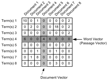
Consider a Corpus C of D documents {d1,d2…..dD} and N unique tokens extracted out of the corpus C. The N tokens will form our dictionary and the size of the Count Vector matrix M will be given by D X N. Each row in the matrix M contains the frequency of tokens in document D(i).
Let us understand this using a simple example.
D1: He is a lazy boy. She is also lazy.
D2: Neeraj is a lazy person.
The dictionary created may be a list of unique tokens(words) in the corpus =[‘He’,’She’,’lazy’,’boy’,’Neeraj’,’person’]
Here, D=2, N=6
The count matrix M of size 2 X 6 will be represented as –
| He | She | lazy | boy | Neeraj | person | |
| D1 | 1 | 1 | 2 | 1 | 0 | 0 |
| D2 | 0 | 0 | 1 | 0 | 1 | 1 |
Now, a column can also be understood as word vector for the corresponding word in the matrix M. For example, the word vector for ‘lazy’ in the above matrix is [2,1] and so on.Here, the rows correspond to the documents in the corpus and the columns correspond to the tokens in the dictionary. The second row in the above matrix may be read as – D2 contains ‘lazy’: once, ‘Neeraj’: once and ‘person’ once.
Now there may be quite a few variations while preparing the above matrix M. The variations will be generally in-
Below is a representational image of the matrix M for easy understanding.
This is another method which is based on the frequency method but it is different to the count vectorization in the sense that it takes into account not just the occurrence of a word in a single document but in the entire corpus. So, what is the rationale behind this? Let us try to understand.
Common words like ‘is’, ‘the’, ‘a’ etc. tend to appear quite frequently in comparison to the words which are important to a document. For example, a document A on Lionel Messi is going to contain more occurences of the word “Messi” in comparison to other documents. But common words like “the” etc. are also going to be present in higher frequency in almost every document.
Ideally, what we would want is to down weight the common words occurring in almost all documents and give more importance to words that appear in a subset of documents.
TF-IDF works by penalising these common words by assigning them lower weights while giving importance to words like Messi in a particular document.
So, how exactly does TF-IDF work?
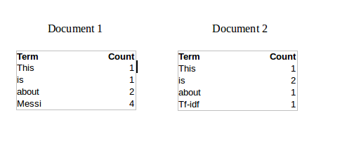
Consider the below sample table which gives the count of terms(tokens/words) in two documents.
Now, let us define a few terms related to TF-IDF.
TF = (Number of times term t appears in a document)/(Number of terms in the document)
So, TF(This,Document1) = 1/8
TF(This, Document2)=1/5
It denotes the contribution of the word to the document i.e words relevant to the document should be frequent. eg: A document about Messi should contain the word ‘Messi’ in large number.
IDF = log(N/n), where, N is the number of documents and n is the number of documents a term t has appeared in.
where N is the number of documents and n is the number of documents a term t has appeared in.
So, IDF(This) = log(2/2) = 0.
So, how do we explain the reasoning behind IDF? Ideally, if a word has appeared in all the document, then probably that word is not relevant to a particular document. But if it has appeared in a subset of documents then probably the word is of some relevance to the documents it is present in.
Let us compute IDF for the word ‘Messi’.
IDF(Messi) = log(2/1) = 0.301.
Now, let us compare the TF-IDF for a common word ‘This’ and a word ‘Messi’ which seems to be of relevance to Document 1.
TF-IDF(This,Document1) = (1/8) * (0) = 0
TF-IDF(This, Document2) = (1/5) * (0) = 0
TF-IDF(Messi, Document1) = (4/8)*0.301 = 0.15
As, you can see for Document1 , TF-IDF method heavily penalises the word ‘This’ but assigns greater weight to ‘Messi’. So, this may be understood as ‘Messi’ is an important word for Document1 from the context of the entire corpus.
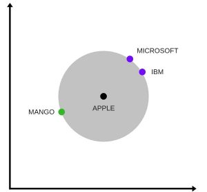
The big idea – Similar words tend to occur together and will have similar context for example – Apple is a fruit. Mango is a fruit.
Apple and mango tend to have a similar context i.e fruit.
Before I dive into the details of how a co-occurrence matrix is constructed, there are two concepts that need to be clarified – Co-Occurrence and Context Window.
Co-occurrence – For a given corpus, the co-occurrence of a pair of words say w1 and w2 is the number of times they have appeared together in a Context Window.
Context Window – Context window is specified by a number and the direction. So what does a context window of 2 (around) means? Let us see an example below,
| Quick | Brown | Fox | Jump | Over | The | Lazy | Dog |
The green words are a 2 (around) context window for the word ‘Fox’ and for calculating the co-occurrence only these words will be counted. Let us see context window for the word ‘Over’.
| Quick | Brown | Fox | Jump | Over | The | Lazy | Dog |
Now, let us take an example corpus to calculate a co-occurrence matrix.
Corpus = He is not lazy. He is intelligent. He is smart.
| He | is | not | lazy | intelligent | smart | |
| He | 0 | 4 | 2 | 1 | 2 | 1 |
| is | 4 | 0 | 1 | 2 | 2 | 1 |
| not | 2 | 1 | 0 | 1 | 0 | 0 |
| lazy | 1 | 2 | 1 | 0 | 0 | 0 |
| intelligent | 2 | 2 | 0 | 0 | 0 | 0 |
| smart | 1 | 1 | 0 | 0 | 0 | 0 |
Let us understand this co-occurrence matrix by seeing two examples in the table above. Red and the blue box.
Red box- It is the number of times ‘He’ and ‘is’ have appeared in the context window 2 and it can be seen that the count turns out to be 4. The below table will help you visualise the count.
| He | is | not | lazy | He | is | intelligent | He | is | smart |
| He | is | not | lazy | He | is | intelligent | He | is | smart |
| He | is | not | lazy | He | is | intelligent | He | is | smart |
| He | is | not | lazy | He | is | intelligent | He | is | smart |
While the word ‘lazy’ has never appeared with ‘intelligent’ in the context window and therefore has been assigned 0 in the blue box.
Variations of Co-occurrence Matrix
Let’s say there are V unique words in the corpus. So Vocabulary size = V. The columns of the Co-occurrence matrix form the context words. The different variations of Co-Occurrence Matrix are-
But, remember this co-occurrence matrix is not the word vector representation that is generally used. Instead, this Co-occurrence matrix is decomposed using techniques like PCA, SVD etc. into factors and combination of these factors forms the word vector representation.
Let me illustrate this more clearly. For example, you perform PCA on the above matrix of size VXV. You will obtain V principal components. You can choose k components out of these V components. So, the new matrix will be of the form V X k.
And, a single word, instead of being represented in V dimensions will be represented in k dimensions while still capturing almost the same semantic meaning. k is generally of the order of hundreds.
So, what PCA does at the back is decompose Co-Occurrence matrix into three matrices, U,S and V where U and V are both orthogonal matrices. What is of importance is that dot product of U and S gives the word vector representation and V gives the word context representation.

Pre-requisite: This section assumes that you have a working knowledge of how a neural network works and the mechanisms by which weights in an NN are updated. If you are new to Neural Network, I would suggest you go through this awesome article by Sunil to gain a very good understanding of how NN works.
So far, we have seen deterministic methods to determine word vectors. But these methods proved to be limited in their word representations until Mitolov etc. el introduced word2vec to the NLP community. These methods were prediction based in the sense that they provided probabilities to the words and proved to be state of the art for tasks like word analogies and word similarities. They were also able to achieve tasks like King -man +woman = Queen, which was considered a result almost magical. So let us look at the word2vec model used as of today to generate word vectors.
Word2vec is not a single algorithm but a combination of two techniques – CBOW(Continuous bag of words) and Skip-gram model. Both of these are shallow neural networks which map word(s) to the target variable which is also a word(s). Both of these techniques learn weights which act as word vector representations. Let us discuss both these methods separately and gain intuition into their working.
The way CBOW work is that it tends to predict the probability of a word given a context. A context may be a single word or a group of words. But for simplicity, I will take a single context word and try to predict a single target word.
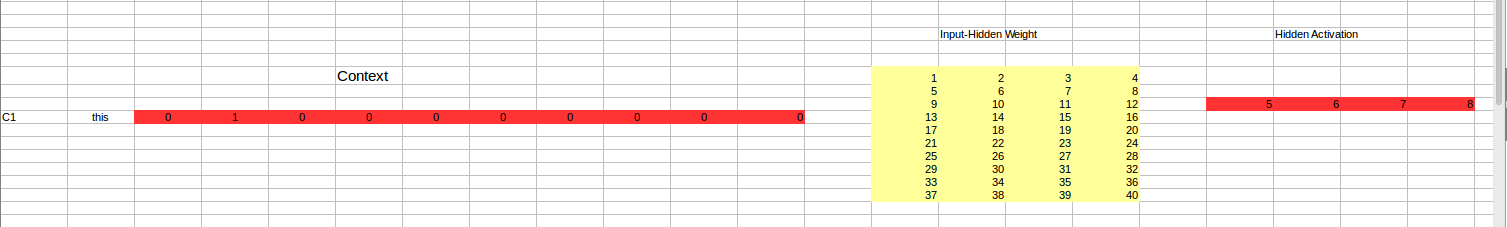
Suppose, we have a corpus C = “Hey, this is sample corpus using only one context word.” and we have defined a context window of 1. This corpus may be converted into a training set for a CBOW model as follow. The input is shown below. The matrix on the right in the below image contains the one-hot encoded from of the input on the left.
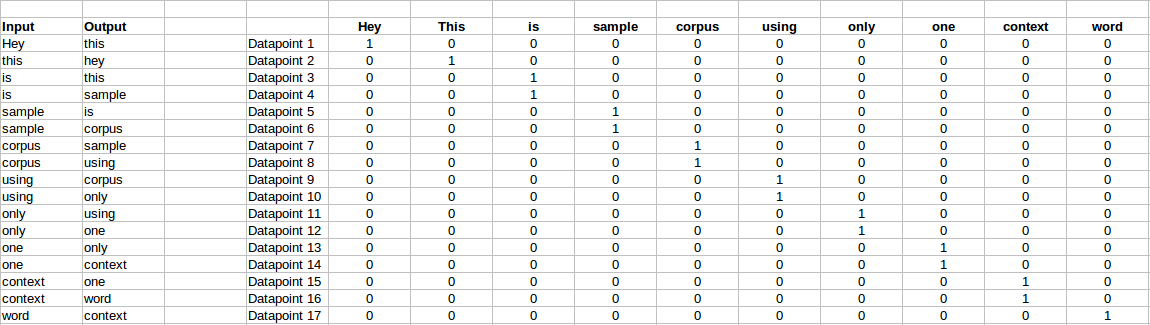
The target for a single datapoint say Datapoint 4 is shown as below
| Hey | this | is | sample | corpus | using | only | one | context | word |
| 0 | 0 | 0 | 1 | 0 | 0 | 0 | 0 | 0 | 0 |
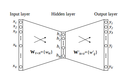
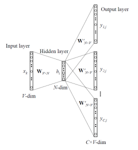
This matrix shown in the above image is sent into a shallow neural network with three layers: an input layer, a hidden layer and an output layer. The output layer is a softmax layer which is used to sum the probabilities obtained in the output layer to 1. Now let us see how the forward propagation will work to calculate the hidden layer activation.
Let us first see a diagrammatic representation of the CBOW model.
The matrix representation of the above image for a single data point is below.
The flow is as follows:
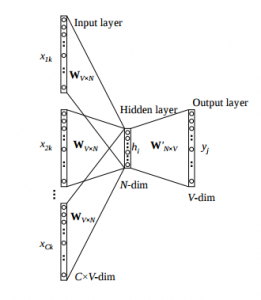
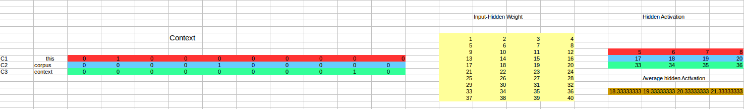
We saw the above steps for a single context word. Now, what about if we have multiple context words? The image below describes the architecture for multiple context words.
Below is a matrix representation of the above architecture for an easy understanding.
The image above takes 3 context words and predicts the probability of a target word. The input can be assumed as taking three one-hot encoded vectors in the input layer as shown above in red, blue and green.
So, the input layer will have 3 [1 X V] Vectors in the input as shown above and 1 [1 X V] in the output layer. Rest of the architecture is same as for a 1-context CBOW.
The steps remain the same, only the calculation of hidden activation changes. Instead of just copying the corresponding rows of the input-hidden weight matrix to the hidden layer, an average is taken over all the corresponding rows of the matrix. We can understand this with the above figure. The average vector calculated becomes the hidden activation. So, if we have three context words for a single target word, we will have three initial hidden activations which are then averaged element-wise to obtain the final activation.
In both a single context word and multiple context word, I have shown the images till the calculation of the hidden activations since this is the part where CBOW differs from a simple MLP network. The steps after the calculation of hidden layer are same as that of the MLP as mentioned in this article – Understanding and Coding Neural Networks from scratch.
The differences between MLP and CBOW are mentioned below for clarification:
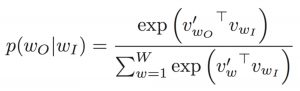
wo : output word
wi: context words
2. The gradient of error with respect to hidden-output weights and input-hidden weights are different since MLP has sigmoid activations(generally) but CBOW has linear activations. The method however to calculate the gradient is same as an MLP.
Skip – gram follows the same topology as of CBOW. It just flips CBOW’s architecture on its head. The aim of skip-gram is to predict the context given a word. Let us take the same corpus that we built our CBOW model on. C=”Hey, this is sample corpus using only one context word.” Let us construct the training data.
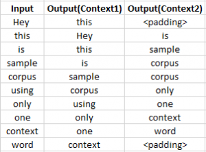
The input vector for skip-gram is going to be similar to a 1-context CBOW model. Also, the calculations up to hidden layer activations are going to be the same. The difference will be in the target variable. Since we have defined a context window of 1 on both the sides, there will be “two” one hot encoded target variables and “two” corresponding outputs as can be seen by the blue section in the image.
Two separate errors are calculated with respect to the two target variables and the two error vectors obtained are added element-wise to obtain a final error vector which is propagated back to update the weights.
The weights between the input and the hidden layer are taken as the word vector representation after training. The loss function or the objective is of the same type as of the CBOW model.
The skip-gram architecture is shown below.
For a better understanding, matrix style structure with calculation has been shown below.
Let us break down the above image.
Input layer size – [1 X V], Input hidden weight matrix size – [V X N], Number of neurons in hidden layer – N, Hidden-Output weight matrix size – [N X V], Output layer size – C [1 X V]
In the above example, C is the number of context words=2, V= 10, N=4
This is an excellent interactive tool to visualise CBOW and skip gram in action. I would suggest you to really go through this link for a better understanding.
Since word embeddings or word Vectors are numerical representations of contextual similarities between words, they can be manipulated and made to perform amazing tasks like-
model.similarity('woman','man')0.73723527model.doesnt_match('breakfast cereal dinner lunch';.split())'cereal'model.most_similar(positive=['woman','king'],negative=['man'],topn=1)queen: 0.508model.score(['The fox jumped over the lazy dog'.split()])0.21Below is one interesting visualisation of word2vec.
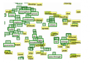
The above image is a t-SNE representation of word vectors in 2 dimension and you can see that two contexts of apple have been captured. One is a fruit and the other company.
5. It can be used to perform Machine Translation.
The above graph is a bilingual embedding with chinese in green and english in yellow. If we know the words having similar meanings in chinese and english, the above bilingual embedding can be used to translate one language into the other.
We are going to use google’s pre-trained model. It contains word vectors for a vocabulary of 3 million words trained on around 100 billion words from the google news dataset. The downlaod link for the model is this. Beware it is a 1.5 GB download.
from gensim.models import Word2Vec
#loading the downloaded model
model = Word2Vec.load_word2vec_format('GoogleNews-vectors-negative300.bin', binary=True, norm_only=True)
#the model is loaded. It can be used to perform all of the tasks mentioned above.
# getting word vectors of a word
dog = model['dog']
#performing king queen magic
print(model.most_similar(positive=['woman', 'king'], negative=['man']))#picking odd one out
print(model.doesnt_match("breakfast cereal dinner lunch".split()))#printing similarity index
print(model.similarity('woman', 'man'))We will be training our own word2vec on a custom corpus. For training the model we will be using gensim and the steps are illustrated as below.
word2Vec requires that a format of list of list for training where every document is contained in a list and every list contains list of tokens of that documents. I won’t be covering the pre-preprocessing part here. So let’s take an example list of list to train our word2vec model.
sentence=[[‘Neeraj’,’Boy’],[‘Sarwan’,’is’],[‘good’,’boy’]]
#training word2vec on 3 sentencesmodel = gensim.models.Word2Vec(sentence, min_count=1,size=300,workers=4)
Let us try to understand the parameters of this model.
sentence – list of list of our corpus
min_count=1 -the threshold value for the words. Word with frequency greater than this only are going to be included into the model.
size=300 – the number of dimensions in which we wish to represent our word. This is the size of the word vector.
workers=4 – used for parallelization
#using the model

#The new trained model can be used similar to the pre-trained ones.
#printing similarity index
print(model.similarity('woman', 'man'))Now, its time to take the plunge and actually play with some other real datasets. So are you ready to take on the challenge? Accelerate your NLP journey with the following Practice Problems:
 | Practice Problem: Identify the Sentiments | Identify the sentiment of tweets |
 | Practice Problem : Twitter Sentiment Analysis | To detect hate speech in tweets |
Word Embeddings is an active research area trying to figure out better word representations than the existing ones. But, with time they have grown large in number and more complex. This article was aimed at simplying some of the workings of these embedding models without carrying the mathematical overhead. If you feel think that I was able to clear some of your confusion, comment below. Any changes or suggestions would be welcomed.
A. Word embeddings are texts converted into numbers in order to feed the data into machine learning models.
A. Word embeddings are broadly classified into 2: frequency-based embedding and prediction-based embedding.
A. Frequency-based embedding deals with 3 types of vectors: count vector, TF-IDF vector, and co-occurrence vector.
A word embedding algorithm represents words as vectors in a continuous space, enhancing language processing in NLP. Notable examples include Word2Vec and GloVe.
Note: We also have a video course on Natural Language Processing covering many NLP topics including bag of words, TF-IDF, and word embeddings. Do check it out!
Lorem ipsum dolor sit amet, consectetur adipiscing elit,


Very nicely explained... Had read somewhere on tuning the word matrix further ... will post the link shortly!!
Sure and Thank You.
Very nice article
Thank You.
excellent summary
Thank You.
Very good article. .It helped me to better understand word2vec. .thanks
Thank You.
Nice article. Although there is an inconsistency in section 2.1.1. In your written example you say documents = rows and terms = columns, but the visualization of M that you show has that switched. Am I wrong in thinking that the visualization is wrong and that if matters that documents are assigned to rows and terms are assigned to columns?
@Zach Smith.... It doesn't matter in this case. The entries i.e the occurrences of terms in a document are still going to be the same.
great article. thank you
Thank You.
Great Article. Does each word have two vector representation...one representation for word acting as context word and other representation for word acting as central word??
Each word has just one vector representation. You can use it either as a context or an input. Thanks.
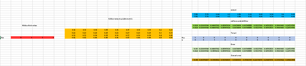
Thanks for this nice article! I have been waiting for word embedding related detailed article since long. However, I have a query. In your excel calculations for skip gram, is the matrix multiplication shown for hidden activation row and each column from hidden output weight matrix? If yes, I am getting some different answer for output matrix. Can you please check? Or am I missing something?
Yes, the calculation shown is between hidden activation and hidden-output matrix. You can paste your output vector below and I can have a look.
Thanks for the nice article!
Great explanation. I do have a question about the co-occurrence matrix, though. Shouldn't the red box contain the number 5 for a context size of 2 (around)? Around the word 'intelligent' you have two instances of "He is" on the left and the right of 'intelligent'. You only count the 'is' on the left and 'He' on the right. Why is that?
Read the co-occurrence matrix for the red box as - For the word 'He', how many times has 'is' appeared in the 2-context window. The word 'intelligent' has nothing to do with the co-occurrence of 'he' and 'is'.
Great job! Very good flow and well explained. I do have one question though regarding the output layer. For your case, you should have two vectors representing the context words we wish to "predict" once training is complete. When performing the multiplication between the input hidden weight matrix and hidden output weight matrix, your entries for each output vector are identical. This makes sense to me since you are using the same hidden output weight matrix and same input hidden matrix value for each of the output layers. So, after applying the softmax function, the vectors should still be identical right? A post from SO(last post of the question: https://stats.stackexchange.com/questions/194011/how-does-word2vecs-skip-gram-model-generate-the-output-vectors) states that all C distributions are different, because of the softmax function. This doesn't make sense to me since given the format of softmax, each element inside of one of the C output layers would just be (for the case of the first element): element(1)/(element1+..element10). Does the change occur after the first error propogation? A lecture from Stanford also displays the output layer (before softmax) to NOT be identical for each of the C windows(https://www.youtube.com/watch?v=ERibwqs9p38, time=39.22). I'm very confused on this as I've had many conflicting opinions. Thanks so much for your help!
Yes, the change occurs after the first error propagation.
very very amazing explaintion....many things gather about yourself...yes realy i enjoy it
Hi NSS. Really great tutorial with respect to word embeddings, the best I've seen by far. However there's still a question baffling me all the time. In the CBOW algorithm, you point out that 'The weight between the hidden layer and the output layer is taken as the word vector representation of the word'. But under the Skip-Gram section, you then say, 'The weights between the input and the hidden layer are taken as the word vector representation after training'. Could you please explain a little bit about what's the difference between the two weight matrices when it comes to word embedding representations?
It is more of an empirical choice. You can choose either weights but generally what people use is the weight matrix near to the single word as vector representation. For example in CBOW, the output is a single word so weight matrix between hidden and output is preferred while in skip gram, input word is a single word, so the weight matrix between input and hidden is preferred.
NSS, Thanks for the great explanation. I have a question regarding the skip gram model. The skip gram model will produce different vector representations for the different semantic contexts a word is used in. I did not follow how that will be the case. What I understood is, since we are getting the word representations from the hidden to output weight matrix, we will have only one representation for each of the words, i.e., the column in the hidden to output matrix corresponding to the one hot column of the word we are considering. It will be great if you can clarify this.
Hi NSS, thank you for this great article. Would you mind elaborating on this sentence: "Being probabilistic is nature, it is supposed to perform superior to deterministic methods(generally)." ? It seems to me that Word2vec is deterministic in the sense that there is no stochastic unit in the model. It's only that CBOW uses softmax to compute probabilities of the different potential outcomes. On a same corpus, if you run CBOW twice, will you get the same vector values ? If no, why ? To what extent do probabilistic models perform superior ? Thank you so much for your clarifications
hi NSS, thanks a lot for such detailed document, I have one question for now, how have to calculated the output layer in your explanation. I want to understand input/output excel snippet in CBOW as well SKIP GRAM, could you please explain that part.
Heya, Great article! I have a question for the co-occurence matrix. If we "place" our window on the middle "is", wouldn't "lazy" and "intelligent" appear in the same window and therefore the count in the co-occurence matrix should be 1? Let me try to visualize it: [ *lazy* He __is__ *intelligent* He ]
Hi, thank you for the great article. The thing I am unable to comprehend is how Prediction based Vector can be used for word similarity/or how the similar words ends up having the same vector so we can use cosine/any similarity mechanisms. As you mentioned in the article it is predicting the target word from contexts or vice versa so it is contextual to that sentence. Lets say we have 2 sentences i) do you accept credit cards and ii) do you take credit cards? will take = accept if trained by skip-gram?
Hey, this really helped. Well, the hidden-output weight & input-hidden weight are adjusted to minimize the error, Finally, the hidden-output weight is used as the word vector representation but what about the input-hidden weights? Is there any importance of them too?
Count Vector in nlp only gives a matrix with numbers. But How could we know for which term is the value assigned in a document?
Very Nice article, Can u kindly explain me one thing: In the CBOW algorithm, you point out that ‘The weight between the hidden layer and the output layer is taken as the word vector representation of the word’, The Matrix size is (N X V) , but the vector representation is of size N. Are we going to make average of all the rows before creating vectors.
NIce explaintion! But how to decide the value of weight?
If I want to do an nlp task in hindi, will pretrained vectors from Wikipedia or GoogleNews be better or my own corpus( 6000 data points each class) ? Also, my hindi data set comes from Twitter and mostly revolves around current topics like politics, iphone event, movies etc.
Very good explanation about word2vecs. Also illustration is wonderful. However, I want to learn how you can acquire this knowledge. :) Please make more content like this.
Hey bro, that's really an awesome article, very well explained!!! The original paper is hard to understand for NLP beginners. Thank you!!!
Hey hi ! Thanks for the great and clear explanation, there is one doubt though, In the skip-gram model diagram, we have final two vectors since context window size is 2, now in the excel sheet it has been shown that both the vectors are same, but there softmax probabilities are different, how could that be ? My overall question is that how we get vectors for each of the words in the context ?
Excellent resource. Clear and very well organized. I was trying to understand the concepts for two days and this is the best one. Thanks.
Thanks for the great intuition tutorial . I have one question regarding context window. For the sample corpus C = “Hey, this is sample corpus using only one context word.” in CBOW and Skip-Gram models, where context window is 1, the input-outputs you have shown are [hey, this],[this, hey], [is, this], [is, sample] but why we skipped [this, is] Is it for any specific reason. Please help me if I'm understanding the context window wrongly.
Very nice article thanks a lot.....
Very good article.
Thanks for the tutorial! I have a question regarding the context window and CBOW. For the context window=1 case, consider the word 'is'. You mentioned the input-output pairs as "is this" and "is sample" for "this is sample" in the one-hot encoding table. However, shouldn't it be "this is" and "sample is" instead since the input should be the context words (which are 'this' and 'sample' in this case) and the output, 'is'? Thank you!
Thanks man for this great contribution, really by far the best tutorial to lean Word2Vec and related concepts. The amazing thing about your explanation is that you have provided a comprehensive understanding of the concepts yet in a simplest possible way.
I have a basic question - more to do with maths or physics meaning of the word "vector" Physics or math defun says vector is an abstract construct that has two peoprtties - one magnitude and other direction. Using vectors defined thus we can use vector representation for physical quantities like displacement, velocity, acceleration, force etc. As opposed to this a property such as mass is a scalar qty having only magnitude. So fsr so good abt vectors in matha and newtonian physics. If we come back machine learning and NLP - it seems that a vector is single dimension array containing some numbers. Its a matrix of one dimension. Why are calling this array as vector ? Is there anything i am missing or is it just a matter of choice for someone to call array or single dimension matix as vector
Excellent brief for beginners! Thanks for sharing! May I ask a question about different semantics? You said above that "Skip-gram model can capture two semantics for a single word. i.e it will have two vector representations of Apple. One for the company and other for the fruit." Does it mean "apple" will have only one vector representation, but this vector representation capture two semantics? Can't the CBOW model do this?
Thanks for the very good explanation about word vectors and related information. I have one question related to Co-Occurrence matrix. In the example you have mentioned an NxN Co-Occurrence matrix models a context window of size 2. How to consider a bigger context window, for example, 5 ?
Thanks for your detailed article. I think it will be very useful for people who are planning to study NLP like me. Thank you!
I feel you are a bit lazy or afraid of explaining clearly, please take your time to explain in details. When you worked that hard then please make it 100%. Else no need to contribute to noise.
Really great article. I have one question: after download 'GoogleNews-vectors-negative300.bin', where should I save it so Python will load it automatically?
I am very happy to see that your tutorial places all types of word representations under the name 'embeddings'.. That clears much confusion. Thanks :)
Congratulations for such a detailed, well exampled, illustrated and step-by-step explanation of word embedding! I really understood and enjoyed this article tremendously! Many other articles describe these processes at such a high level that understanding is much more difficult.
Very clear explanation! I have one question about skip-gram predicting Apple. I understand Apple's word vector is kind of between fruit and company. I do not understand why skip-gram would generate two vector representations for Apple as you mentioned in the article. I think each word is supposed to have only one vector representation.
I had the same question as sharath chandra. Is the omission of [this, is] a typo? Otherwise, great tutorial!
This is a naive explanation of embeddings friends. This site is pretty much a ad-hack on 2-grams data analysis and machine learning. Please stop bullshitting people with non-degree'd explanations. You do a disservice to all.
Thanks for the article it helps build a base for word embedding.
Thank you for the article. But I am still unsure about one point about Skip Gram model's outputs: So all C output vectors are always same with each other? And C one-hot vectors(that represent truth) are compared with the same skip-gram output vector? (During single training iteration I mean) Will be really grateful if someone clears it up
That is a really great article ! things are simple yet powerful and clear
Thank you. Very minor edit In CBOW example this, is is missing as the third data point.
Thanks Saul for the feedback. I have updated the article
A very nice and thoughtful article. In 2.1.3, I could not understand how and why HE and IS were counted in the 3rd example.Can you please explain ?? Thanks
2.1.3 Co-Occurrence Matrix with a fixed context window In this section : Shouldn't the matrix be like :- features features he is not lazy intelligent smart he 0 3 1 1 1 1 is 0 0 1 1 1 1 not 0 0 0 1 0 0 lazy 0 0 0 0 0 0 intelligent 0 0 0 0 0 0 smart 0 0 0 0 0 0
Very nice article. Thank you so much. How can I download to my computer? Thank you
Hey NSS, Very Useful Article Bro :-) Thank You For Sharing It
There is a row missing in CBOW for "this" -> "is" and so the data points are off by 1. Nice job btw.
Thanks so much 4your nice article. I wanna to use skip gram for text doc summarization with gensim and cluster for semantic part. Please,May i know how to use and include sentences scoring in python code ?