Introduction
I love cricket as much as I love data science. A few years back (on 16 November 2013 to be precise), my favorite cricketer – Sachin Tendulkar retired from International Cricket. I spent that entire day reading articles and blogs about him on the web.
By the end of the day, I had read close to 50 articles about him. Interestingly, while I was reading these articles – none of the websites suggested me articles outside of Sachin or cricket. Was it a co-incidence? Surely not.
I was being suggested the next article based on what I was currently reading. The technique behind this process is known as “Information Retrieval”.
In this article, I would take you through the basics of Information Retrieval and two common algorithms used to implement it, KNN and KD Tree. By end of this article, you will be able to create your own information retrieval systems, which can be implemented in any digital library / search.
Let’s get going!
Table of Contents
- What is Information Retrieval?
- Where is Information Retrieval used?
- KNN for Information Retrieval
- Improvement over KNN: KD Trees for Information Retrieval
- Explanation of KD Trees
- Implementation of KD Trees
- Advantages and Disadvantages of KD trees
What is Information Retrieval?
In the past few decades, the availability of cheap and effective storage devices and information systems has prompted the rapid growth of graphical and textual databases. Information collection and storage efforts have become easier, but the effort required to retrieve relevant information has become significantly greater, especially in large-scale databases. This situation is critical for textual databases, with so much of textual information around us – for instance business applications (e.g., manuals, newsletters, and electronic data interchanges), scientific applications (e.g., electronic community systems and scientific databases) etc.

To aid the users to access these databases and extract the relevant knowledge or documents, Information Retrieval is used.
Information Retrieval (IR) is the process by which a collection of data is represented, stored, and searched for the purpose of knowledge discovery as a response to a user request (query). This process involves various stages initiating with representing data and ending with returning relevant information to the user. The intermediate stage includes filtering, searching, matching and ranking operations. The main goal of information retrieval system (IRS) is to “find the relevant information or a document that satisfies user’s information needs”
Where is Information Retrieval used?
Use Case 1: Digital Library
A digital library is a library in which collection of data are stored in digital formats and accessible by computers. The digital content may be stored locally, or accessed remotely via computer networks. A digital library is a type of information retrieval system.
Use Case 2: Search Engine
A search engine is one of the most the practical applications of information retrieval techniques to large scale text collections.
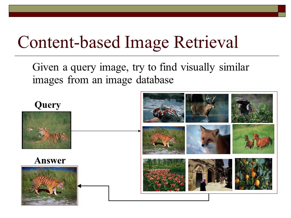
Use Case 3: Image retrieval
An image retrieval system is a computer system for browsing, searching and retrieving images from a large database of digital images.
Very famous example of image retrieval system is https://reverse.photos/ which uses image as the search query and returns similar images.

KNN for Information Retrieval
One of the most common algorithms that most of the Data scientists use for retrieval of information is KNN. K Nearest Neighbour (KNN) is one of the simplest algorithms that calculates the distance between the query observation and each data point in the train dataset and finds the K closest observations.
When we use Nearest neighbour search algorithm, it compares all the data points with the mentioned query point and finds the closest points.
There are many ways in which we can find the distance between two data points. Most commonly used distance metrics are “Euclidean distance” and “Hamming distance”.
This research paper focuses on them.
Imagine a situation where you have thousands of queries, and every time the algorithm compares the query point with all the data points. Isn’t it very computationally intensive?
Also, greater the data points, higher will be the amount of computation needed. Obviously!

So, KNN search has O(N) time complexity for each query where N= Number of data points. For KNN with K neighbor search, the time complexity will be O(log(K)*N) only if we maintain a priority queue to return the closest K observations. You can read more about KNN here.
So, for a dataset with millions of rows and thousands of queries, KNN seems to be computationally very demanding. So is there any alternative to KNN which uses similar approach but can be time efficient also?
KD Tree is one such algorithm which uses a mixture of Decision trees and KNN to calculate the nearest neighbour(s).
Improvement over KNN: KD Trees for Information Retrieval
KD-trees are a specific data structure for efficiently representing our data. In particular, KD-trees helps organize and partition the data points based on specific conditions.
Let’s say we have a data set with 2 input features. We can represent our data as-

Now, we’re going to be making some axis aligned cuts, and maintaining lists of points that fall into each one of these different bins.


And what this structure allows us to do as we’re going to show, is efficiently prune our search space so that we don’t have to visit every single data point.
Now the question arises of how to draw these cuts?
- One option is to split at the median value of the observations that are contained in the box.
- You could also split at the centre point of the box, ignoring the spread of data within the box
Then a question is when do you stop?
There are a couple of choices that we have.
- One is you can stop if there are fewer than a given number of points in the box. Let’s say m data points left.
- Or if a minimum width to the box has been achieved.
So again, this second criteria would ignore the actual data in the box whereas the first one uses facts about the data to drive the stocking criterion. We can use the same distance metrics(“Euclidean distance” and “Hamming distance”) that we used while implementing KNN.
Intuitive Explanation of KD Trees
Suppose we have a data set with only two features.
| X | Y | |
| Data point 0 | 0.54 | 0.93 |
| Data point 1 | 0.96 | 0.86 |
| Data point 2 | 0.42 | 0.67 |
| Data point 3 | 0.11 | 0.53 |
| Data point 4 | 0.64 | 0.29 |
| Data point 5 | 0.27 | 0.75 |
| Data point 6 | 0.81 | 0.63 |
Let’s split data into two groups.
We do it by comparing x with mean of max and min value.
Value = (Max + Min)/2
= (0.96 + 0.11)/2
= 0.53


At each node we will save 3 things.
- Dimension we split on
- Value we split on
- Tightest bounding box which contains all the points within that node.
| Tight bounds | X | Y |
| Node 1 | 0.11 <= X <= 0.42 | 0.53 <= Y <= 0.75 |
| Node 2 | 0.54 <= X <= 0.96 | 0.29 <= Y <= 0.93 |
Similarly dividing the structure into more parts on the basis of alternate dimensions until we get maximum 2 data points in a Node.


So now we plotted the points and divided them into various groups.
Let’s say now we have a query point ‘Q’ to which we have to find the nearest neighbor.

Using the tree we made earlier, we traverse through it to find the correct Node.

When using Node 3 to find the Nearest Neighbor.

But we can easily see, that it is in fact not the Nearest neighbor to the Query point.

We now traverse one level up, to Node 1. We do this because the nearest neighbor may not necessarily fall into the same node as the query point.
Do we need to inspect all remaining data points in Node 1 ?
We can check this by checking if the tightest box containing all the points of Node 4 is closer than the current near point or not.

This time, the bounding box for Node 4 lies within the circle, indicating that Node 4 may contain a point that’s closer to the query.

When we calculate the distance of the points within the Node 4 and previous closest point with the query point, we find that point lying above the query point is actually the nearest neighbor within the given points.

We now traverse one level up, to Root.
Do we need to inspect all remaining data points in Node 2 ?
We can check this by checking if the tightest box containing all the points of Node 2 is closer than the current Near point or not.

We can see that the Tightest box is far from the current Nearest point. Hence, we can prune that part of the tree.


Since we’ve traversed the whole tree, we are done: data point marked is indeed the true nearest neighbour of the query.
Implementation of KD Trees
For the implementation of KD Tree, we will use the most common form of IR ie Document Retrieval. Based on the current document, document retrieval returns the most similar document(s) to the user.
We will use the dataset which consists of articles on famous personalities. We would implement KD Tree to help us retrieve articles most similar to that of the “Barack Obama”.
You can download the dataset in the form of csv from here.
In [1]:
#Importing libraries
import pandas as pd
import numpy as np
import nltk
In [2]:
#Reading first 2000 rows of the dataset
people = pd.read_csv('people_data.csv',nrows =2000)
In [4]:
#Using countvectoriser to count the freq of occurence of each word
from sklearn.feature_extraction.text import CountVectorizer
count_vect = CountVectorizer()
X_train_counts = count_vect.fit_transform(people.text)
In [5]:
#Using tf-idf to reduce the effect of common words
from sklearn.feature_extraction.text import TfidfTransformer
tfidf_transformer = TfidfTransformer()
X_train_tfidf = tfidf_transformer.fit_transform(X_train_counts)
In [6]:
#Using tfidf as a feature
people['tfidf']=list(X_train_tfidf.toarray())
In [8]:
#Importing KDTree
from sklearn.neighbors import KDTree
kdt = KDTree(people['tfidf'].tolist(), leaf_size=3)
In [9]:
#Using KDTree to find 3 articles similar to that of Barack Obama
dist, idx = kdt.query(people['tfidf'][people['name']=='Barack Obama'].tolist(), k=3)
In [10]:
#Indices of 3 nearest articles
idx[0]
Out[10]:
array([ 32, 0, 1177])
In [11]:
#Nearest neighbour 1
people['name'][32]
Out[11]:
'Barack Obama'
In [12]:
#Nearest neighbour 2
people['name'][0]
Out[12]:
'Bill Clinton'
In [13]:
#Nearest neighbour 3
people['name'][1177]
Out[13]:
'Donald Fowler'
Hence we can see that articles of Bill Clinton and Donald Flower who share the same field of politics as Barack Obama are similar.
Advantages and Disadvantages of KD trees
Advantages of KD Trees
So now we look at the advantages of KD Tree :
- So to begin with, the first thing we have to do when we have a query point, is that we traverse all the way down to a leaf node. So we’re going to go all the way down to the depth of the tree. In the worst case, we would have to traverse N nodes, the worst case being when, because of the structure of the problem we’re not able to prune anything at all.
- The complexity range is anywhere from on the order of log N, if we can do lots of pruning, everything gets pruned, all the way to on the order of N, if we can’t do any pruning.
- Remember that order N was the same complexity as our KNN search. So, if we’re just going to do a single nearest neighbour query and if we got really unlucky about the structure of the data, we might take a penalty over a KNN search. But in many cases, we can actually have significant gains in efficiency and time.
Disadvantages of KD Tree
Well, KD-trees are really cool. They’re a very intuitive way to think about storing data, and as we saw, they could lead to help us find relevant information way sooner.
But there are few issues.
- KD-trees are not the simplest things to implement. You have to structure out this tree, and it can be pretty challenging to do that.

- As the features of our data, i.e. dimensionality increases, we might get a poor performance in terms of efficiency of nearest neighbor search using KD-trees. This is because we won’t be able to prune many partitions as in high dimension, the radius of our nearest neighbour would intersect many different partitions, which would force us to look for a better nearest neighbour among the points stored in them. So we won’t be able to prune many of these partitions, and what ends up happening is that we would have to search many partitions which completely defeats the purpose of using KD-trees. As displayed in the above image, no of inspections would increase exponentially as the dimensionality of the dataset increase.
End Notes
KD Tree can prove to be a better Retrieval algorithm on a specific Dataset that matches its condition. Though there are more models such as Locality Sensitive Hashing which can overcome its limitations. We shall explore them as well in the upcoming articles.
Did you find the article useful? Do you plan to use KD Tree or LSH in near future in Python or R? If yes, share with us how you plan to go about it.
Gurchetan1000 Singh
27 Aug, 2021
Budding Data Scientist from MAIT who loves implementing data analytical and statistical machine learning models in Python. I also understand big data technology like Hadoop and Alteryx.


Powerful article. Where can I study this?
Hey James Glad that you liked the article !! You can refer to "Intro to Statistical Learning", a book by Trevor Hastie for more insights. Coursera also offers a course on Clustering and Retrieval by Univ Of Washington. You can watch it's videos for detailed explanation.
Nice and easy explanation !
Excellent article worth reading and it is very informative
R methods of writing available ?
Hey James I only use Python for implementing ML. Hence I have no idea regarding the R code. If you manage to implement it in future, do share with us.
Why Value = (Max + Min)/2 instead of Value = (Max - Min)/2 ? Is there some advantage to adding Max and Min over Max - Min?
Hey Jarad The idea is to take the average value which can equally divide the datasets into equal parts. Instead of taking the average of all datapoints, we consider only the extremes for calculating the average. So Max+Min/2 sounds intuitively more correct as it will give some value in between while Max-Min/2 might not.
Nice one thanks for sharing
Awesome article
Have you guys explored K-D-B tree, hB-tree or BKD tree? I think BKD takes care of some of the limitations of KD tree.