An Introduction To Non Stationary Time Series In Python
Introduction
The applications of predicting household electricity consumption, estimating road traffic, and forecasting stock prices all share a common thread—they rely on time series data. Without accounting for the ‘time’ component, accurately predicting these outcomes would be virtually impossible. As data generation continues to surge, mastering time series forecasting emerges as a pivotal skill for data scientists.
However, delving into time series analysis reveals a multifaceted landscape. One of the fundamental challenges lies in addressing non-stationarity within the data. Non-stationary trends are prevalent in most datasets, presenting hurdles for forecasting models. Erratic spikes and fluctuations can disrupt the predictive accuracy of models, underscoring the critical importance of making time series data stationary.
In this article, we embark on an exploration of time series analysis, navigating through concepts such as autoregressive behavior, autocorrelation function (ACF), moving average, and random walk. With insights drawn from econometrics and a keen understanding of stochastic and deterministic trends, we delve into strategies to tame non-stationarity. By unraveling the complexities of time series data, we aim to equip data scientists with the tools necessary to extract meaningful insights and drive informed decision-making.
Learning Outcomes
- Proficiency in analyzing stock price data using time series analysis techniques to uncover seasonal components, trends, and underlying patterns.
- Understanding the concept of stationarity in time series analysis, including recognizing second-order stationarity and distinguishing series with no trend.
- Familiarity with statistical tests like ADF and KPSS to assess stationarity and interpret their results in the context of significance levels.
- Mastery of techniques such as differencing and transformation to address non-linear trends and make time series data suitable for modeling.
- Recognition of white noise and its significance in time series analysis, aiding in the identification of random fluctuations versus meaningful patterns in data science applications.
This article was published as a part of the Data Science Blogathon.
Table of contents
Understanding Stationarity
Stationarity is one of the most important concepts you will come across when working with time series data. A stationary series is one in which the properties – mean, variance and covariance, do not vary with time.
Let us understand this using an intuitive example. Consider the three plots shown below:
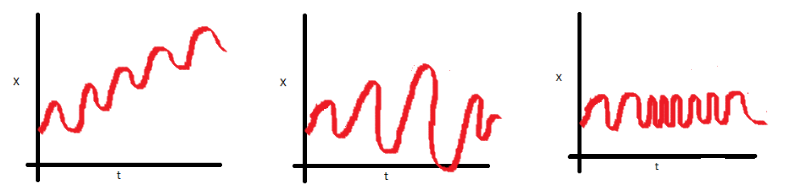
- In the first plot, we can clearly see that the mean varies (increases) with time which results in an upward trend. Thus, this is a non-stationary series. For a series to be classified as stationary, it should not exhibit a trend.
- Moving on to the second plot, we certainly do not see a trend in the series, but the variance of the series is a function of time. As mentioned previously, a stationary series must have a constant variance.
- If you look at the third plot, the spread becomes closer as the time increases, which implies that the covariance is a function of time.
The three examples shown above represent non-stationary time series. Now look at a fourth plot:
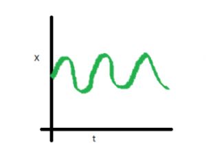
Consider this: In a stationary time series, mean, variance, and covariance remain constant over time. Predicting future values is easier with a stationary series, enhancing the precision of statistical models. Thus, for effective predictions, ensuring stationarity is crucial. To recap, a stationary time series maintains consistent properties regardless of time. In the upcoming section, we’ll delve into methods for verifying stationarity in a given series.
Loading The Data
In the upcoming sections, I’ll introduce methods for assessing time series data stationarity and strategies for handling non-stationary series. Additionally, I’ll share Python code for each technique. You can access the dataset we’ll utilize via this link: AirPassengers. Before we go ahead and analyze our dataset, let’s load and preprocess the data first.
Before we go ahead and analyze our dataset, let’s load and preprocess the data first.
#loading important libraries
import pandas as pd
import matplotlib.pyplot as plt
%matplotlib inline

#reading the dataset
train = pd.read_csv('AirPassengers.csv')

#preprocessing
train.timestamp = pd.to_datetime(train.Month , format = '%Y-%m')
train.index = train.timestamp
train.drop('Month',axis = 1, inplace = True)

#looking at the first few rows
#train.head()
| #Passengers | |
|---|---|
| Month | |
| 1949-01-01 | 112 |
| 1949-02-01 | 118 |
| 1949-03-01 | 132 |
| 1949-04-01 | 129 |
| 1949-05-01 | 121 |
Methods to Check Stationarity
The next step is to determine whether a given series is stationary or not and deal with it accordingly. This section looks at some common methods which we can use to perform this check.
Visual test
Consider the plots we used in the previous section. We were able to identify the series in which mean and variance were changing with time, simply by looking at each plot. Similarly, we can plot the data and determine if the properties of the series are changing with time or not.
train['#Passengers'].plot()
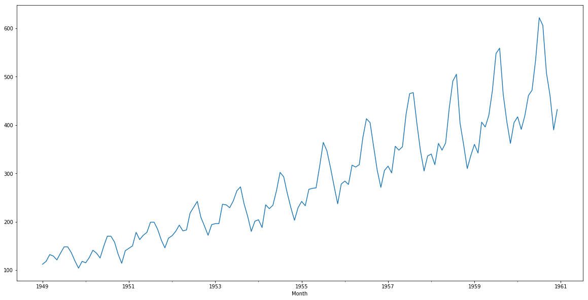
Although its very clear that we have a trend (varying mean) in the above series, this visual approach might not always give accurate results. It is better to confirm the observations using some statistical tests.
Statistical test
Instead of going for the visual test, we can use statistical tests like the unit root stationary tests. Unit root indicates that the statistical properties of a given series are not constant with time, which is the condition for stationary time series. Here is the mathematics explanation of the same :
Suppose we have a time series :
yt = a*yt-1 + ε t
where yt is the value at the time instant t and ε t is the error term. In order to calculate yt we need the value of yt-1, which is :
yt-1 = a*yt-2 + ε t-1
If we do that for all observations, the value of yt will come out to be:
yt = an*yt-n + Σεt-i*ai
If the value of a is 1 (unit) in the above equation, then the predictions will be equal to the yt-n and sum of all errors from t-n to t, which means that the variance will increase with time. This is knows as unit root in a time series. We know that for a stationary time series, the variance must not be a function of time. The unit root tests check the presence of unit root in the series by checking if value of a=1.
Below are the two of the most commonly used unit root stationary tests:
ADF (Augmented Dickey Fuller) Test
The Dickey Fuller test is one of the most popular statistical tests. It can be used to determine the presence of unit root in the series, and hence help us understand if the series is stationary or not. The null and alternate hypothesis of this test are:
Null Hypothesis: The series has a unit root (value of a =1)
Alternate Hypothesis: The series has no unit root.
If we fail to reject the null hypothesis, we can say that the series is non-stationary. This means that the series can be linear or difference stationary (we will understand more about difference stationary in the next section).
#define function for ADF test
from statsmodels.tsa.stattools import adfuller
def adf_test(timeseries):
    #Perform Dickey-Fuller test:
    print ('Results of Dickey-Fuller Test:')
    dftest = adfuller(timeseries, autolag='AIC')
    dfoutput = pd.Series(dftest[0:4], index=['Test Statistic','p-value','#Lags Used','Number of Observations Used'])
    for key,value in dftest[4].items():
       dfoutput['Critical Value (%s)'%key] = value
    print (dfoutput)

#apply adf test on the series
adf_test(train['#Passengers'])
Results of ADF test: The ADF tests gives the following results – test statistic, p value and the critical value at 1%, 5% , and 10% confidence intervals. The results of our test for this particular series are:
Results of Dickey-Fuller Test:
Test Statistic                   0.815369
p-value                          0.991880
#Lags Used                      13.000000
Number of Observations Used    130.000000
Critical Value (1%)             -3.481682
Critical Value (5%)             -2.884042
Critical Value (10%)            -2.578770
dtype: float64
Test for stationarity: If the test statistic is less than the critical value, we can reject the null hypothesis (aka the series is stationary). When the test statistic is greater than the critical value, we fail to reject the null hypothesis (which means the series is not stationary).
In our above example, the test statistic > critical value, which implies that the series is not stationary. This confirms our original observation which we initially saw in the visual test.
KPSS (Kwiatkowski-Phillips-Schmidt-Shin) Test
KPSS is another test for checking the stationarity of a time series (slightly less popular than the Dickey Fuller test). The null and alternate hypothesis for the KPSS test are opposite that of the ADF test, which often creates confusion.
The authors of the KPSS test have defined the null hypothesis as the process is trend stationary, to an alternate hypothesis of a unit root series. We will understand the trend stationarity in detail in the next section. For now, let’s focus on the implementation and see the results of the KPSS test.
Null Hypothesis: The process is trend stationary.
Alternate Hypothesis: The series has a unit root (series is not stationary).
#define function for kpss test
from statsmodels.tsa.stattools import kpss
#define KPSS
def kpss_test(timeseries):
    print ('Results of KPSS Test:')
    kpsstest = kpss(timeseries, regression='c')
    kpss_output = pd.Series(kpsstest[0:3], index=['Test Statistic','p-value','Lags Used'])
    for key,value in kpsstest[3].items():
    kpss_output['Critical Value (%s)'%key] = value
print (kpss_output)
Results of KPSS test: Following are the results of the KPSS test – Test statistic, p-value, and the critical value at 1%, 2.5%, 5%, and 10% confidence intervals. For the air passengers dataset, here are the results:
Test for stationarity: If the test statistic is greater than the critical value, we reject the null hypothesis (series is not stationary). If the test statistic is less than the critical value, if fail to reject the null hypothesis (series is stationary). For the air passenger data, the value of the test statistic is greater than the critical value at all confidence intervals, and hence we can say that the series is not stationary.
I usually perform both the statistical tests before I prepare a model for my time series data. It once happened that both the tests showed contradictory results. One of the tests showed that the series is stationary while the other showed that the series is not! I got stuck at this part for hours, trying to figure out how is this possible. As it turns out, there are more than one type of stationarity.
So in summary, the ADF test has an alternate hypothesis of linear or difference stationary, while the KPSS test identifies trend-stationarity in a series.
Types of Stationarity
Let us understand the different types of stationarities and how to interpret the results of the above tests.
- Strict Stationary: A strict stationary series satisfies the mathematical definition of a stationary process. For a strict stationary series, the mean, variance and covariance are not the function of time. The aim is to convert a non-stationary series into a strict stationary series for making predictions.
- Trend Stationary: A series that has no unit root but exhibits a trend is referred to as a trend stationary series. Once the trend is removed, the resulting series will be strict stationary. The KPSS test classifies a series as stationary on the absence of unit root. This means that the series can be strict stationary or trend stationary.
- Difference Stationary: A time series that can be made strict stationary by differencing falls under difference stationary. ADF test is also known as a difference stationarity test.
It’s always better to apply both the tests, so that we are sure that the series is truly stationary. Let us look at the possible outcomes of applying these stationary tests.
- Case 1: Both tests conclude that the series is not stationary -> series is not stationary
- Case 2: Both tests conclude that the series is stationary -> series is stationary
- Case 3: KPSS = stationary and ADF = not stationary -> trend stationary, remove the trend to make series strict stationary
- Case 4: KPSS = not stationary and ADF = stationary -> difference stationary, use differencing to make series stationary
Making a Time Series Stationary
Now that we are familiar with the concept of stationarity and its different types, we can finally move on to actually making our series stationary. Always keep in mind that in order to use time series forecasting models, it is necessary to convert any non-stationary series to a stationary series first.
Differencing
In this method, we compute the difference of consecutive terms in the series. Differencing is typically performed to get rid of the varying mean. Mathematically, differencing can be written as:
yt‘ = yt – y(t-1)
where yt is the value at a time t
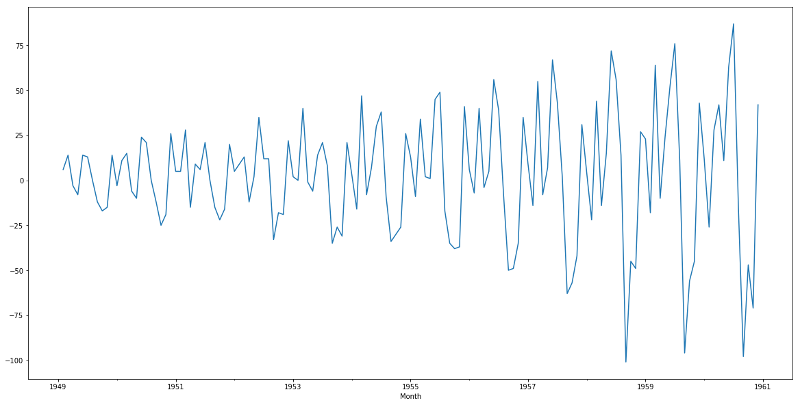
Applying differencing on our series and plotting the results:
train['#Passengers_diff'] = train['#Passengers'] - train['#Passengers'].shift(1)
train['#Passengers_diff'].dropna().plot()
Seasonal Differencing
In seasonal differencing, instead of calculating the difference between consecutive values, we calculate the difference between an observation and a previous observation from the same season. For example, an observation taken on a Monday will be subtracted from an observation taken on the previous Monday. Mathematically it can be written as:
yt‘ = yt – y(t-n)
n=7
train['#Passengers_diff'] = train['#Passengers'] - train['#Passengers'].shift(n)
Transformation
Transformations are used to stabilize the non-constant variance of a series. Common transformation methods include power transform, square root, and log transform. Let’s do a quick log transform and differencing on our air passenger dataset:
train['#Passengers_log'] = np.log(train['#Passengers'])
train['#Passengers_log_diff'] = train['#Passengers_log'] - train['#Passengers_log'].shift(1)
train['#Passengers_log_diff'].dropna().plot()
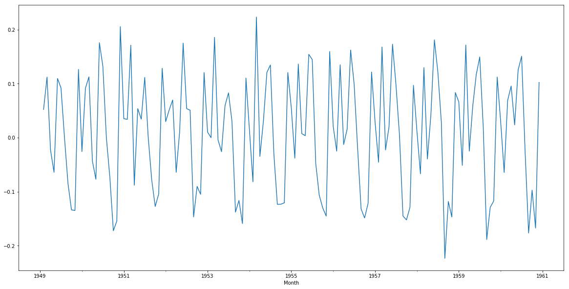
As you can see, this plot is a significant improvement over the previous plots. You can use square root or power transformation on the series and see if they come up with better results. Feel free to share your findings in the comments section below!
Conclusion
Mastering time series analysis is vital for effective forecasting and modeling of temporal data. Through this guide, we’ve explored the importance of stationarity and methods for assessing it, such as visual inspection and statistical tests like ADF and KPSS. We’ve also discussed different types of stationarity and techniques like differencing and transformation to make non-stationary data suitable for modeling. Understanding autocorrelation, residual analysis, and model validation are essential for accurate forecasting. By applying these techniques, analysts can extract valuable insights from time series data and make informed decisions.
Key Take Away
- Time series analysis plays a crucial role in understanding and forecasting stock price movements, enabling data scientists to identify seasonal components and trends.
- Identifying second-order stationarity helps distinguish between stationary series with no trend and those exhibiting non-linear patterns, aiding in model selection and interpretation.
- Utilizing statistical tests like ADF and KPSS helps determine the stationarity of time series data and set significance levels for model validation.
- Techniques such as differencing and transformation are essential for addressing non-linear trends and making time series data suitable for modeling and analysis.
- Recognizing white noise in time series data is vital for distinguishing random fluctuations from meaningful patterns, enhancing the effectiveness of data-driven decision-making processes.
Frequently Asked Questions
A. A stationary process is one whose statistical properties, such as mean, variance, and autocorrelation, do not change over time. Non-stationary time series data, on the other hand, exhibit statistical properties that change over time.
A. Difference between a stationary and a nonstationary random process is:
Stationary Process: A stationary process has constant statistical properties over time. These properties include mean, variance, and autocorrelation. In a stationary process, these properties do not change with time shifts.
Non-stationary Process: A non-stationary process has statistical properties that vary over time. This variation can be in the mean, variance, or other moments of the distribution. Non-stationary processes often exhibit trends, seasonal patterns, or other systematic changes.
A. Handling non-stationary time series typically involves transforming the data to make it stationary or modeling the non-stationarity explicitly. Common techniques include:
Detrending: Removing trend components from the data to make it stationary. This can involve techniques like linear regression or differencing.
Differencing: Taking differences between consecutive observations to remove trends or seasonal patterns.
Transformation: Applying mathematical transformations such as logarithms or square roots to stabilize the variance.
Decomposition: Decomposing the time series into its trend, seasonal, and residual components and modeling each separately.
Modeling: Using models that explicitly account for non-stationarity, such as autoregressive integrated moving average (ARIMA) models or seasonal decomposition of time series (STL).
The media shown in this article is not owned by Analytics Vidhya and is used at the Author’s discretion
An avid reader and blogger who loves exploring the endless world of data science and artificial intelligence. Fascinated by the limitless applications of ML and AI; eager to learn and discover the depths of data science.


Great post. For differencing, you can also use the diff method on pandas Series and DataFrame objects.
Thanks Carl!
I will call it "A Great Introduction to Handling a Non-Stationary Time Series in Python". Thanks Aishwarya
Thank you Miguel!
Hi Aishwarya, which test would be better to check the stationarity, ADF Test or the KPSS test?
Hi Shreyansh, It's preferred to apply both the tests to check if the series is stationary. In case the tests give contradictory results, you would have to deal with the dataset accordingly (remove trend or perform differencing operation based on the results)
Hi there. I recently come across few articles on transformation of non stationary data and mentioned quite extensive use of the Box Cox transformation technique as an alternative to the log transformation. What is you oppinion on such the approach and what the major use case differences between the Box Cox and log. Thanks Alex
Hi Alex, Log transform is a derivative of box cox transform. If you give the lambda value as 0, it will perform a log transform. The main difference is that unlike log transform, box cox is not restricted to one value. This link shows a table for the transformations performed for different lambda values in box cox.
Thank you for the great article. Between Differencing / Seasonal Differencing & Log transformation, looks like log transformation provides the best result. Could that be the default one to do for most time series data. Thank you
Hi John, Both the transformations are for different purposes. Differencing removes the trend present in the series while log transformation is for handling high variance in the series. Based on the dataset, you can use any one or both of the methods to make the series stationary.
Good article. Quick question. Once we make it stationary, can we model this as a regression problem using month / Yr and the transformed feature (difference or difference) as the target variable? Best,
Hi Henry, I haven't tried it before but I see no reason why this cannot be treated as a regression problem. You'll just have to perform reverse of the transformations after you get the results.
Hi Aishwarya, Im afraid that I don't understand. What did you graph after you changes in the transform? Third line seems like it should be: train['#Passengers_log'] = np.sqrt(train['#Passengers_log_diff'].dropna()).plot() How can I invert this so I am graphing the original data
Hey Robert, Thanks for pointing it out, I have updated the code now. Please check.
Nice Article ever!!
Thank you Davis!
please do same kind of analysis of time series forecasting for uni-variate by support vector machine in r.
Hello, Thanks for this wonderful article. I do have a question and I see that I could not answer myself. I do understand that differencing with some lag(1 or 2 which becomes p in ARIMA), taking log and then differencing etc. removes the trend. But then when we fit the data into model, do we need to fit the original data with trend and seasonal components or the data which we obtained after differencing\log which removes the trend. Best Regards Chandan
Hi, Like ADF, is there any other statistical test to identify the timeseries is following a trend or seasonality? Since it will be a manual work to see the plot and say(trend or seasonality) for 1k different products./ So, I want a statistical test like ADF which will identify the trend or seasonality even if the datapoints are less for each product (say for each product datapoints < 14) Thankyou!
Beautifully explained the different aspects involved.
Hi Aishwara, Thanks for this great post. I was wondering if you got case 3 and case 4 mixed up. You said the following: Case 3: KPSS = stationary and ADF = not stationary -> trend stationary, remove the trend to make series strict stationary Case 4: KPSS = not stationary and ADF = stationary -> difference stationary, use differencing to make series stationary In case 3, when ADF gives non-stationary result, shouldn't we use differencing to make the series strict stationary? And vice versa for case 4?
Thank you so much for such a great article. I've earned a lot knowledge and also courage to keep digging in this field. I wish you all the best!