A Comprehensive Guide to Time Series Analysis and Forecasting

This article was published as a part of the Data Science Blogathon.

Introduction

Time Series Analysis and Forecasting is a very pronounced and powerful study in data science, data analytics and Artificial Intelligence. It helps us to analyse and forecast or compute the probability of an incident, based on data stored with respect to changing time. For example, let us suppose you have visited a clinic due to some chest pain and want to get an electrocardiogram (ECG) test done to see if your heart is healthy functioning. The ECG graph produced is a time-series data where your Heart Rate Variability (HRV) with respect to time is plotted, analysing which the doctor can suggest crucial measures to take care of your heart and reduce the risk of stroke or heart attacks. Time Series is used widely in healthcare analytics, geospatial analysis, weather forecasting, and to forecast the future of data that changes continuously with time!

What is Time Series Analysis in Machine Learning?

Time-series analysis is the process of extracting useful information from time-series data to forecast and gain insights from it. It consists of a series of data that varies with time, hence continuous and non-static in nature. It may vary from hours to minutes and even seconds (milliseconds to microseconds). Due to its non-static and continuous nature, working with time-series data is indeed difficult even today!

As time-series data consists of a series of observations taken in sequences of time, it is entirely non-static in nature.

Time Series – Analysis Vs. Forecasting

The Time Series Integrants

Any time-series problem or data can be broken down or decomposed into several integrants, which can be useful for performing analysis and forecasting. Transforming time series into a series of integrants is called Time Series Decomposition.

A quick thing worth mentioning is that the integrants are broken further into 2 types-

1. Systematic — components that can be used for predictive modelling and occur recurrently. Level, Trend, and Seasonality come under this category.

2. Non-systematic — components that cannot be used for predictive modelling directly. Noise comes under this category.

The original time series data is hence split or decomposed into 5 parts-

1. Level — The most common integrant in every time series data is the level. It is nothing but the mean or average value in the time series. It has 0 variances when plotted against itself.

2. Trend — The linear movement or drift of the time series which may be increasing, decreasing or neutral. Trends are observable over positive(increasing) and negative(decreasing) and even linear slopes over the entire range of time.

3. Seasonality — Seasonality is something that repeats over a lapse of time, say a year. An easy way to get an idea about seasonality- seasons, like summer, winter, spring, and monsoon, which come and go in cycles throughout a specified period of time. However, in terms of data science, seasonality is the integrant that repeats at a similar frequency.

Note — If seasonality doesn’t occur at the same frequency, we call it a cycle. A cycle does not have any predefined and fixed signal or frequency is very uncertain, in terms of probability. It may sometimes be random, which poses a great challenge in forecasting.

4. Noise — A irregularity or noise is a randomly occurring integrant, and it’s optional and arrives under observation if and only if the features are not correlated with each other and, most importantly, variance is the similar across the series. Noise can lead to dirty and messy data and hinder forecasting, hence noise removal or at least reduction is a very important part of the time series data pre-processing stage.

5. Cyclicity — A particular time-series pattern that repeats itself after a large gap or interval of time, like months, years, or even decades.

The Time Series Forecasting Applications

Time series analysis and forecasting are done on automating a variety of tasks, such as-

1. Weather Forecasting
2. Anomaly Forecasting
3. Sales Forecasting
4. Stock Market Analysis
5. ECG Analysis
6. Risk Analysis

and many more!

Time Series Components Combinatorics

A time-series model can be represented by 2 methodologies-

The Additive Methodology — 

When the time series trend is a linear relationship between integrants, i.e., the frequency (width) and amplitude(height) of the series are the same, the additive rule is applied.

Additive methodology is used when we have a time series where seasonal variation is linear or constant over timestamps.

It can be represented as follows-

y(t) or x(t) = level + trend + seasonality + noise

where the model y(multivariate) or x(univariate) is a function of time t.

The Multiplicative Methodology — 

When the time series is not a linear relationship between integrants, then modelling is done following the multiplicative rule.

The multiplicative methodology is used when we have a time series where seasonal variation increases with time — which may be exponential or quadratic.

It is represented as-

y(t) or x(t)= Level * Trend * Seasonality * Noise

Deep-Dive into Supervised Time-Series Forecasting

Supervised learning is the most used domain-specific machine learning, and hence we will focus on supervised time series forecasting.

This will contain various detailed topics to ensure that readers at the end will know how to-

1. Load time series data and use descriptive statistics to explore it
2. Scale and normalize time series data for further modelling
3. Extracting useful features from time-series data (Feature Engineering)
4. Checking the stationarity of the time series to reduce it
5. ARIMA and Grid-search ARIMA models for time-series forecasting
6. Heading to deep learning methods for more complex time-series forecasting (LSTM and bi-LSTMs)

So without further ado, let’s begin!

Load Time Series Data and Use Descriptive Statistics to Explore it

For the easy and quick understanding and analysis of time-series data, we will work on the famous toy dataset named ‘Daily Female Births Dataset’.

Get the dataset downloaded from here.

Importing necessary libraries and loading the data –

import numpy
import pandas
import statmodels
import matplotlib.pyplot as plt
import seaborn as sns
data = pd.read_csv(‘daily-total-female-births-in-cal.csv’, parse_dates = True, header = 0, squeeze=True)
data.head()

This is the output we get-

1959–01–01 35
1959–01–02 32
1959–01–03 30
1959–01–04 31
1959–01–05 44
Name: Daily total female births in California, 1959, dtype: int64

Note —Remember, it is required to use ‘parse_dates’ because it converts dates to datetime objects that can be parsed, header=0 which ensures the column named is stored for easy reference, and squeeze=True which converts the data frame of single object elements into a scalar.

Exploring the Time-Series Data –

print(data.size) #output-365

(a) Carry out some descriptive statistics —

print(data.describe())

Output —

count 365.000000
mean 41.980822
std 7.348257
min 23.000000
25% 37.000000
50% 42.000000
75% 46.000000
max 73.000000

(b) A look at the time-series distribution plot —

pyplot.plot(series)
pyplot.show()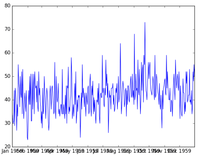

Scale and Normalize Time Series Data for Further Modelling

A normalized data scales the numeric features in the training data in the range of 0 and 1 so that gradient descent and loss optimization is fast and efficient and converges quickly to the local minima. Interchangeably known as feature scaling, it is crucial for any ML problem statement.

Let’s see how we can achieve normalization in time-series data.

For this purpose, let’s pick a highly fluctuating time-series data — the minimum daily temperatures data. Grab it here!

Let’s have a look at the extreme fluctuating nature of the data —

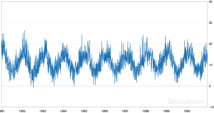
It is seen that it has a strong seasonality integrant. Hence, scaling is important to remove seasonal integrants, and it leads to crisp relationship establishment between independent and target features!

To normalize a feature, Scikit-learn’s MinMaxScaler is too handy! If you want to generate original data points after prediction, an inverse_transform() function is also provided by this awesome built-in function!

Here goes the normalization code —

# import necessary libraries
import pandas
from sklearn.preprocessing import MinMaxScaler
# load and sanity check the data
data = read_csv(‘daily-minimum-temperatures-in-me.csv’, parse_dates = True, header = 0, squeeze=True, index_col=0)
print(data.head())
#convert data into matrix of row-col vectors
values = data.values
values = values.reshape((len(values), 1))
# feature scaling
scaler = MinMaxScaler(feature_range=(0, 1))
#fit the scaler with the train data to get min-max values
scaler = scalar.fit(values)
print(‘Min: %f, Max: %f’ % (scaler.data_min_, scaler.data_max_))
# normalize the data and sanity check
normalized = scaler.transform(values)
for i in range(5):
 print(normalized[i])
# inverse transform to obtain original values
original_matrix= scaler.inverse_transform(normalized)
for i in range(5):
 print(original_matrix[i])

Let’s have a look at what we got –

See how the values have scaled!

Note — In our case, our data does not have outliers present and hence a MinMaxScaler solves the purpose well. In the case where you have an unsupervised learning approach, and your data contains outliers, it is better to go for standardization, which is more robust than normalization, as normalization scales the data close to the mean which doesn’t handle or include outliers leading to a poor model. Standardization, on the other hand, takes large intervals with a standard deviation value of 1 and a mean of 0, thus outlier handling is robust.

More on that here!

Extracting Useful Features from Time-Series Data (Feature Engineering)

Framing data into a supervised learning problem simply deals with the task of handling and extracting useful features and discarding irrelevant features to make the model robust and cost-efficient.

We already know that supervised learning problems have 2 types of features — the independents (x) and dependent/target(y). Hence, how better the target value is achieved depends on how well we choose and engineer the independent features.

You must know by now that time-series data has two columns, timestamp, and its respective value. So, it is very self-explanatory that in the time series problem, the independent feature is time and the dependent feature is value.

Now let us look at what are the features that need to be engineered into these input and output values so that the inherent relationship between these two variables is established to make the forecasting as good as possible.

The features which are extremely important to model the relationship between the input and output variables in a time series are —

1. Descriptive Statistical Features — Quite straightforward as it sounds, calculating the statistical details and summary of any data is extremely important. Mean, Median, Standard Deviation, Quantiles, and min-max values. These come extremely handy while in tasks such as outlier detection, scaling and normalization, recognizing the distribution, etc.

2. Window Statistic Features — Window features are a statistical summary of different statistical operations upon a fixed window size of previous timestamps. There are, in general, 2 ways to extract descriptive statistics from windows. They are

(a) Rolling Window Statistics: The rolling window focuses on calculating rolling means or what we conventionally call Moving Average, and often other statistical operations. This calculates summary statistics (mostly mean) across values within a specific sliding window, and then we can assign these as features in our dataset.

Let, the mean at timestamp t-1 is x and t-2 be y, so we find the average of x and y to predict the value at timestamp t+1. The rolling window hence takes a mean of 2 values to predict the 3rd value. After that is done, the window shifts to the next set of values, and hence the mean is calculated for each window consisting of 2 values. We use rolling window statistics more often when the recent data is more important for forecasting and not previous data.

Let’s see how we can calculate moving or rolling average with a rolling window —

from pandas import DataFrame
from pandas import concat
df = DataFrame(data.values)
tshifts = df.shift(1)
rwin = tshifts.rolling(window=2)
moving_avg = rwin.mean()
joined_df = concat([moving_avg, df], axis=1)
joined_df.columns = [‘mean(t-2,t-1)’, ‘t+1’]
print(joined_df.head(5))

Let’s have a look at what we got —

(b) Expanding Window Statistics: Almost similar to the rolling window, expanding windows takes into account an extra habit of extracting the predicted value as well as all the previous observations, each time it expands. This is beneficial when the previous data is equally important for forecasting as well as the recent data.

Let’s have a quick look at expanding window code-

window = tshifts.expanding()
joined_df2 = concat([rwin.mean(),df.shift(-1)], axis=1)
joined_df2.columns = ['mean', 't+1']
print(joined_df2.head(5))

Let’s have a look at what we got -

3. Lag Features — Lag is simply predicting the value at timestamp t+1, provided we know the value at the previous timestamp, say, t-1. It’s simply distance or lag between two values at 2 different timestamps.

4. Datetime Features — This is simply the conversion of time into its specific components like a month, or day, along with the value of temperature for better forecasting. By doing this, we can gather specific information about the month and day at a particular timestamp for each record.

5. Timestamp Decomposition — Timestamp decomposition includes breaking down the timestamp into subset columns of timestamp for storing unique and special timestamps. Before Diwali or, say, Christmas, the sale of crackers and Santa-caps, fruit-cakes increases exponentially more than at other times of the year. So storing such a special timestamp by decomposing the original timestamp into subsets is useful for forecasting.

Time-series Data Stationary Checks

So, let’s first digest what stationary time-series data is!

Stationary, as the term suggests, is consistent. In time-series, the data if it does not contain seasonality or trends is termed stationary. Any other time-series data that has a specific trend or seasonality, are, thus, non-stationary.

Can you recall, that amongst the two time-series data we worked on, the childbirths data had no trend or seasonality and is stationary. Whereas, the average daily temperatures data, has a seasonality factor and drifts, and hence, it’s non-stationary and hard to model!

Stationarity in time-series is noticeable in 3 types —

(a) Trend Stationary — This kind of time-series data possesses no trend.

(b) Seasonality Stationary — This kind of time-series data possesses no seasonality factor.

(c) Strictly Stationary — The time-series data is strictly consistent with almost no variance to drifts.

Now that we know what stationarity in time series is, how can we check for the same?

Vision is everything. A quick visualization of your time-series data at hand can give a quick eye review of whether the data can be stationary or not. Next in the line comes the statistical summary. A clear look into the summary statistics of the data like min, max, variance, deviation, mean, quantiles, etc. can be very helpful to recognize drifts or shifts in data.

Lets POC this!

So, we take stationary data, which is the handy childbirths data we worked on earlier. However, for the non-stationary data, let’s take the famous airline-passenger data, which is simply the number of airline passengers per month, and prove how they are stationary and non-stationary.

Case 1 — Stationary Proof

import pandas as pd
import matplotlib.pyplot as plt
data = pd.read_csv(‘daily-total-female-births.csv’, parse_dates = True, header = 0, squeeze=True)
data.hist()
plt.show()

Output —

As I said, vision! Look how the visualization itself speaks that it’s a Gaussian Distribution. Hence, stationary!

More curious? Let’s get solid math proof!

X = data.values
seq = round(len(X) / 2)
x1, x2 = X[0:seq], X[seq:]
meanx1, meanx2 = x1.mean(), x2.mean()
varx1, varx2 = x1.var(), x2.var()
print(‘meanx1=%f, meanx2=%f’ % (meanx1, meanx2))
print(‘variancex1=%f, variancex2=%f’ % (varx1, varx2))

Output —

meanx1=39.763736, meanx2=44.185792
variancex1=49.213410, variancex2=48.708651

The mean and variances linger around each other, which clearly shows the data is invariant and hence, stationary! Great.

Case 2— Non-Stationary Proof

import pandas as pd
import matplotlib.pyplot as plt
data = pd.read_csv(‘international-airline-passengers.csv’, parse_dates = True, header = 0, squeeze=True)
data.hist()
plt.show()

Output —

The graph pretty much gives a seasonal taste. Moreover, it is too distorted for a Gaussian tag. Let’s now quickly get the mean-variance gaps.

X = data.values
seq = round(len(X) / 2)
x1, x2 = X[0:seq], X[seq:]
meanx1, meanx2 = x1.mean(), x2.mean()
varx1, varx2 = x1.var(), x2.var()
print(‘meanx1=%f, meanx2=%f’ % (meanx1, meanx2))
print(‘variancex1=%f, variancex2=%f’ % (varx1, varx2))

Output —

meanx1=182.902778, meanx2=377.694444
variancex1=2244.087770, variancex2=7367.962191

Alright, the value gap between mean and variances are pretty self-explanatory to pick the non-stationary kind.

ARMA, ARIMA, and SARIMAX Models for Time-Series Forecasting

A very traditional yet remarkable ‘machine-learning’ way of forecasting a time series is the ARMA (Auto-Regressive Moving Average) and Auto Regressive Integrated Moving Average Model commonly called ARIMA statistical models.

Other than these 2 traditional approaches, we have SARIMA (Seasonal Auto-Regressive Integrated Moving Average) and Grid-Search ARIMA, which we will see too!

So, let’s explore the models, one by one!

ARMA

The ARMA model is an assembly of 2 statistical models — the AR or Auto-Regressive model and Moving Average.

The Auto-Regressive Model estimates any dependent variable value y(t) at a given timestamp t on the basis of lags. Look at the formula below for a better understanding —

Here, y(t) = predicted value at timestamp t, α = intercept term, β = coefficient of lag, and, y(t-1) = time-series lag at timestamp t-1.

So α and β are the model estimators that estimate y(t).

The Moving Average Model plays a similar role, but it does not take the past predicted forecasts into account, as said earlier in rolling average. It rather uses the lagged forecast errors in previously predicted values to predict the future values, as shown in the formula below.

Let’s see how both the AR and MA models perform on the International-Airline-Passengers data.

AR model

AR_model = ARIMA(indexedDataset_logScale, order=(2,1,0))
AR_results = AR_model.fit(disp=-1)
plt.plot(datasetLogDiffShifting)
plt.plot(AR_results.fittedvalues, color='red')
plt.title('RSS: %.4f'%sum((AR_results.fittedvalues - datasetLogDiffShifting['#Passengers'])**2))

The RSS or sum of squares residual is 1.5023 in the case of the AR model, which is kind of dissatisfactory as AR doesn’t capture non-stationarity well enough.

MA Model

MA_model = ARIMA(indexedDataset_logScale, order=(0,1,2))
MA_results = MA_model.fit(disp=-1)
plt.plot(datasetLogDiffShifting)
plt.plot(MA_results.fittedvalues, color='red')
plt.title('RSS: %.4f'%sum((MA_results.fittedvalues - datasetLogDiffShifting['#Passengers'])**2))

The MA model shows similar results to AR, differing by a very small amount. We know our data is non-stationary, so let’s make this RSS score better by the non-stationarity handler AR+I+MA!

ARIMA

Along with the squashed use of the AR and MA model used earlier, ARIMA uses a special concept of Integration(I) with the purpose of differentiating some observations in order to make non-stationary data stationary, for better forecasting. So, it’s obviously better than its predecessor ARMA which could only handle stationary data.

What the differencing factor does is, that it takes into account the difference in predicted values between two timestamps (t and t+1, for example). Doing this helps in achieving a constant mean rather than a highly fluctuating ‘non-stationary’ mean.

Let’s fit the same data with ARIMA and see how well it performs!

ARIMA_model = ARIMA(indexedDataset_logScale, order=(2,1,2))
ARIMA_results = ARIMA_model.fit(disp=-1)
plt.plot(datasetLogDiffShifting)
plt.plot(ARIMA_results.fittedvalues, color='red')
plt.title('RSS: %.4f'%sum((ARIMA_results.fittedvalues - datasetLogDiffShifting['#Passengers'])**2))

Great! The graph itself speaks how ARIMA fits our data in a well and generalized fashion compared to the ARMA! Also, observe how the RSS has dropped to 1.0292 from 1.5023 or 1.4721.

SARIMAX

Designed and developed as a beautiful extension to the ARIMA, SARIMAX or, Seasonal Auto-Regressive Integrated Moving Average with eXogenous factors is a better player than ARIMA in case of highly seasonal time series. There are 4 seasonal components that SARIMAX takes into account.

They are -

 1. Seasonal Autoregressive Component

 2. Seasonal Moving Average Component

 3. Seasonal Integrity Order Component

 4. Seasonal Periodicity

If you are more of a theory conscious person like me, do read more on this here, as getting into the details of the formula is beyond the scope of this article!

Now, let’s see how well SARIMAX performs on seasonal time-series data like the International-Airline-Passengers data.

from statsmodels.tsa.statespace.sarimax import SARIMAX
SARIMAX_model=SARIMAX(train['#Passengers'],order=(1,1,1),seasonal_order=(1,0,0,12))
SARIMAX_results=SARIMAX_model.fit()
preds=SARIMAX_results.predict(start,end,typ='levels').rename('SARIMAX Predictions')
test['#Passengers'].plot(legend=True,figsize=(8,5))
preds.plot(legend=True)

Look how beautifully SARIMAX handles seasonal time series!

Heading to DL Methods for Complex Time-Series Forecasting

One of the very common features of time-series data is the long-term dependency factor. It is obvious that many time-series forecasting works on previous records (the future is forecasted based on previous records, which may be far behind). Hence, ordinary traditional machine learning models like ARIMA, ARMA, or SARIMAX are not capable of capturing long-term dependencies, which makes them poor guys in sequence-dependent time series problems.

To address such an issue, a massively intelligent and robust neural network architecture was proposed which can extraordinarily handle sequence dependence. It was known as Recurrent Neural Networks or RNN.

RNN was designed to work on sequential data like time series. However, a very remarkable pitfall of RNN was that it couldn’t handle long-term dependencies. For a problem where you want to forecast a time series based on a huge number of previous records, RNN forgets the maximum of the previous records which occurred much earlier, and only learns sequences of recent data fed to its neural network. So, RNN was observed to not be up to the mark for NSP (Next Sequence Prediction) tasks in NLP and time series.

To address this issue of not capturing long-term dependencies, a powerful variant of RNN was developed, known as LSTM (Long Short Term Memory) Networks. Unlike RNN, which could only capture short-term sequences/dependencies, LSTM, as its name suggests was observed to learn long as well as short term dependencies. Hence, it was a great success for modelling and forecasting time series data!

Note — Since explaining the architecture of LSTM will be beyond the size of this blog, I recommend you to head over to my article where I explained LSTM in detail!

Let us now take our Airline Passengers’ data and see how well RNN and LSTM work on it!

Imports —

import numpy as np
import pandas as pd
import tensorflow as tf
import matplotlib.pyplot as plt
import sklearn.preprocessing
from sklearn.metrics import r2_score
from keras.layers import Dense, Dropout, SimpleRNN, LSTM
from keras.models import Sequential

Scaling the data to make it stationary for better forecasting — 

minmax_scaler = sklearn.preprocessing.MinMaxScaler()
data['Passengers'] = minmax_scaler.fit_transform(data['Passengers'].values.reshape(-1,1))
data.head()

Scaled data — 

 

Train, test splits (80–20 ratio) — 

split = int(len(data[‘Passengers’])*0.8)

x_train,y_train,x_test,y_test = np.array(x[:split]),np.array(y[:split]),
np.array(x[split:]), np.array(y[split:])

#reshaping data to original shape
x_train = np.reshape(x_train, (split, 20, 1))
x_test = np.reshape(x_test, (x_test.shape[0], 20, 1))

RNN Model — 

model = Sequential()
model.add(SimpleRNN(40, activation="tanh", return_sequences=True, input_shape=(x_train.shape[1],1)))
model.add(Dropout(0.15))
model.add(SimpleRNN(50, return_sequences=True, activation="tanh"))
model.add(Dropout(0.1)) #remove overfitting
model.add(SimpleRNN(10, activation="tanh"))
model.add(Dense(1))
model.summary()

Complie it, fit it and predict— 

model.compile(optimizer="adam", loss="MSE")
model.fit(x_train, y_train, epochs=15, batch_size=50)
preds = model.predict(x_test)

Let me show you a picture of how well the model predicts — 

Pretty much accurate!

LSTM Model — 

model = Sequential()
model.add(LSTM(100, activation="ReLU", return_sequences=True, input_shape=(x_train.shape[1], 1)))
model.add(Dropout(0.2))
model.add(LSTM(80, activation="ReLU", return_sequences=True))
model.add(Dropout(0.2))
model.add(LSTM(50, activation="ReLU", return_sequences=True))
model.add(Dropout(0.2))
model.add(LSTM(30, activation="ReLU"))
model.add(Dense(1))
model.summary()

Complie it, fit it and predict— 

model.compile(optimizer="adam", loss="MSE")

model.fit(x_train, y_train, epochs=15, batch_size=50)
preds = model.predict(x_test)

Let me show you a picture of how well the model predicts —

Here, we can easily observe that RNN does the job better than LSTMs. As it is clearly seen that LSTM works great in training data but bad invalidation/test data, which shows a sign of overfitting!

Hence, try to use LSTM only where there is a need for long-term dependency learning otherwise RNN works good enough.

Conclusion

Cheers on reaching the end of the guide and learning pretty interesting kinds of stuff about Time Series. From this guide, you successfully learned the basics of time series, got a brief idea of the difference between Time Series Analysis and Forecasting subdomains of Time Series, a crisp mathematical intuition on Time Series analysis and forecasting techniques and explored how to work on Time Series problems in Machine Learning and Deep Learning to solve complex problems.

Hope you had fun exploring Time Series with Machine Learning and Deep Learning along with intuition! If you are a curious learner and want to “not” stop learning more, head over to this awesome notebook on time series provided by TensorFlow!

Feel free to follow me on Medium and GitHub for more articles and notebooks on Machine & Deep Learning! Connect with me on LinkedIn if you want to discuss anything regarding this article!

Happy Learning!

The media shown in this article is not owned by Analytics Vidhya and is used at the Author’s discretion.