Mathematics behind Machine Learning – The Core Concepts you Need to Know
Overview
- Here’s an intuitive and beginner friendly guide to the mathematics behind machine learning
- Learn the various math concepts required for machine learning, including linear algebra, calculus, probability and more
Introduction
“What’s the use of learning the mathematics behind machine learning algorithms? We can easily use the widely available libraries available in Python and R to build models!”
I have lost count of the number of times I’ve heard this from amateur data scientists. This fallacy is all too common and has created a false expectation among aspiring data science professionals.
There are primarily two reasons for this in my experience:
- Mathematics is quite daunting, especially for folks coming from a non-technical background. Apply that complexity to machine learning and you’ve got quite an intimidating situation
- As mentioned, a vast array of libraries exist to perform various machine learning tasks so it’s easy to avoid the mathematical part of the field
Let’s get this out of the way right now – you need to understand the mathematics behind machine learning algorithms to become a data scientist. There is no way around it. It is an intrinsic part of a data scientist’s role and every recruiter and experienced machine learning professional will vouch for this.
So this brings us to the question of how? How should we go about learning this? Mathematics for machine learning is an essential aspect of becoming a machine learning master. In this article, we’ll discuss various mathematical concepts, including linear algebra, probability, and more, that you need to know to succeed in the field of machine learning.
Table of Contents
In this article, we will discuss the below topics:
- Difference between the Mathematics Behind Machine Learning and Data Science
- Attitude adjustment for approaching a former enemy
- Linear Algebra for Machine Learning
- Multivariate Calculus for Machine Learning
- Probability for Machine Learning
- Statistics for Machine Learning
So without further ado, let’s dive right into it.
Difference Between the Mathematics Behind Machine Learning and Data Science
One of the most common questions I’m regularly asked by aspiring data scientists is – what’s the different between data science and machine learning? And more to the point, what’s the difference between the mathematics behind these two?
I regularly encounter these questions:
- Where do I use probability in Machine Learning?
- Where do I use Multivariate Calculus in Data Science?
- Where do I use Linear Algebra in Data Science?
Although Data Science and Machine Learning share a lot of common ground, there are subtle differences in their focus on mathematics. The below radar plot encapsulates my point:
Yes, Data Science and Machine Learning overlap a lot but they differ quite a bit in their primary focus. And this subtle difference is often the source of the questions I mentioned above.
In Data Science, our primary goal is to explore and analyse the data, generate hypotheses and test them.
These are often the steps to draw out the hidden inferences in the data which might not observable at first sight. As a result, we have to rigorously rely on the concepts of statistics and probability to compare and conduct hypothesis testing.
On the other hand, Machine learning focuses more on the concepts of Linear Algebra as it serves as the main stage for all the complex processes to take place (besides the efficiency aspect). On the other hand, multivariate calculus deals with the aspect of numerical optimisation, which is the driving force behind most machine learning algorithms.
Data science is generally considered as the prerequisite to machine learning. Think about it – we expect the input data for machine learning algorithms to be clean and prepared with respect to the technique we use. If you are among the ones who are looking to work end-to-end (Data Science + Machine Learning), it will be better to make yourself proficient with the union of the math required for Data Science and Machine Learning.
Attitude Adjustment for Approaching a Former Enemy
If you keep repeating the same thing thing that you’ve done in the past, you will get the results you have always been getting. I’m paraphrasing Albert Einstein’s famous quote here but I’m sure you get the idea!
Many machine learning aspirants make this mistake of following the same methodology as they did during their school days. This means using a pen and paper to grind through the theorems, derivations and questions.

This traditional methodology can’t be any farther from what we want to be following, unless you want to be in a 17th century battle of mathematicians. They challenged each other over a set number of mathematically intriguing questions to be solved by the next day. It sounds glorious but as you can imagine, it’s not the best way to learn a new concept in the 21st century.
So how can you learn mathematics without getting bogged down into the theory?
Mathematics in data science and machine learning is not about crunching numbers, but about what is happening, why it’s happening, and how we can play around with different things to obtain the results we want.
In essence:
We should be more concerned about the intuition and the geometric interpretation of any given expression:
This helps us interpret the meaning behind these mind boggling expressions. All the laborious work of manually working through the problems is not essential, and does not require skill. Working through them using computational libraries like NumPy makes much more sense instead of testing your stamina.
Now, let’s shift our focus to understand why we need to learn these different tributaries of mathematics and what would be a good source to learn it the intuitive way.
Linear Algebra for Machine Learning
Some people consider linear algebra to be the mathematics of the 21st century. I can see the sense in that – linear algebra is the backbone of machine learning and data science which are set to revolutionise every other industry in the coming years.
As I have already discussed before, linear algebra acts as a stage or a platform over which all the machine learning algorithms cook their results.
But why linear algebra?
Linear Algebra acts as the systematic basis of the representation for simultaneous linear equations.
Let’s say we are given two linear equations:
Solving for x and y is pretty easy, right?

We can do it by simply multiplying equation 1 by -2 and then adding both:

As a result, the variable x is eliminated and y is obtained as 9. On back substituting we get the value of x as 0.
The problem here is that this operation requires human intuition to work. Our machines cannot mimic the same intuition. They can only understand data in a certain representation and rules in a set format.

Now, to establish an analogy with data science or machine learning, each equation represents a single observation from the dataset. The left-hand side represents the independent input variables and the right-hand side represents the target dependent variable.
Datasets often contain hundreds and thousands of observations (if not millions), not to mention that there can be a lot of variables to work with. So do you think we can work through the datasets and find the optimum value of x and y manually?
Absolutely not! We would definitely prefer automation for this task. And this is where Linear Algebra comes into play. In a broad sense:
Linear algebra is a systematic representation of the knowledge that a computer can understand and all the operations in linear algebra are systematic rules.
This is the algebraic representation of the problem we solved above. Using the matrix operations (set of rules), we can solve for the values of x and y in the blink of an eye. This is the primary reason linear algebra is a necessity in data science and machine learning. Also, it plays a vital role when it comes to unsupervised techniques like PCA.
To learn linear algebra using the classic intuition and some practice, you cannot go wrong with this (Linear Algebra – Imperial College of London)
Multivariate Calculus for Machine Learning
Most aspiring data science and machine learning professionals often fail to explain where they need to use multivariate calculus. As I mentioned at the start of the article, this is unfortunately an all too common experience.
If you immediately said Gradient Descent, you’re on the right path! But you might need to add on to your existing knowledge.
Multivariate calculus, or partial differentiation to be more precise, is used for the mathematical optimisation of a given function (mostly convex).
But why do we do that? We know that we calculate the partial derivative of some function (cost function or the optimisation function). But how does it help?
Most folks often find the partial derivative but have no idea why they just did that! We need to rectify this immediately.
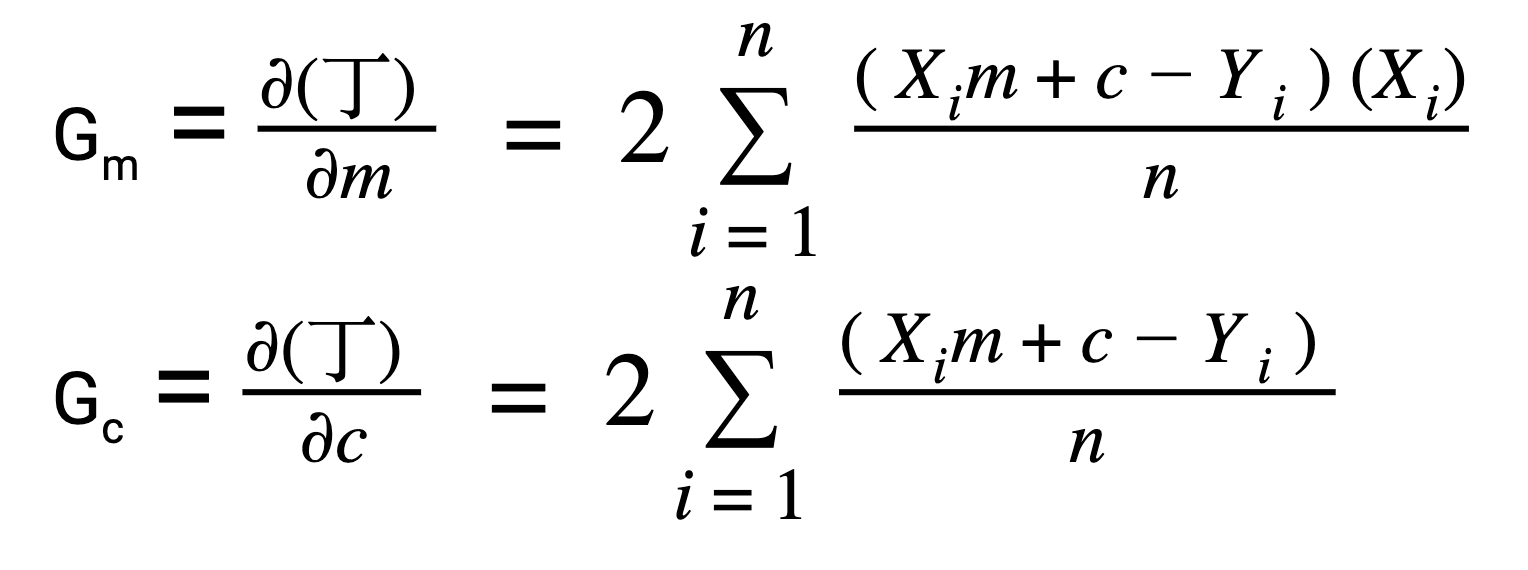
Let’s consider the case of gradient descent. We know the cost function of the gradient descent is given as:
And we calculate the derivatives with respect to the m(slope) and c(intercept) as:
But why only partial derivative? We could have calculated the integral or some other operation. This is because the differentiation gives us the rate of change in the cost function with respect to the cost 丁 with respect to the m and c individually.
But do you know we can represent these individual partial derivatives in a vector form?
This is the algebraic vector representation of the partial derivatives.
I’m sure that most of you must have seen this representation before but did not realize what it signified. This representation is called the Jacobian vector. I personally came across this in my high school days; and yes, it did make my life difficult!
Below are a few excellent resources for learning multivariate calculus. Again, I will emphasise more on the intuition part rather than just cramming up the theorems and rules:
Khan Academy (taught by 3Blue1Brown):
Multivariate Calculus (Imperial College of London):
Probability for Machine Learning
Probability concepts required for machine learning are elementary (mostly), but it still requires intuition. It is often used in the form of distributions like Bernoulli distributions, Gaussian distribution, probability density function and cumulative density function. We use them to carry out hypothesis testing where an understanding of probability is quite essential.
You will find many data scientists, even seasoned veterans, who cannot explain the true meaning of the infamous alpha value and the p-value. They are often treated as some unknown strangers who arrived from Pluto, and nobody even cares to ask. You can learn more p-value here.
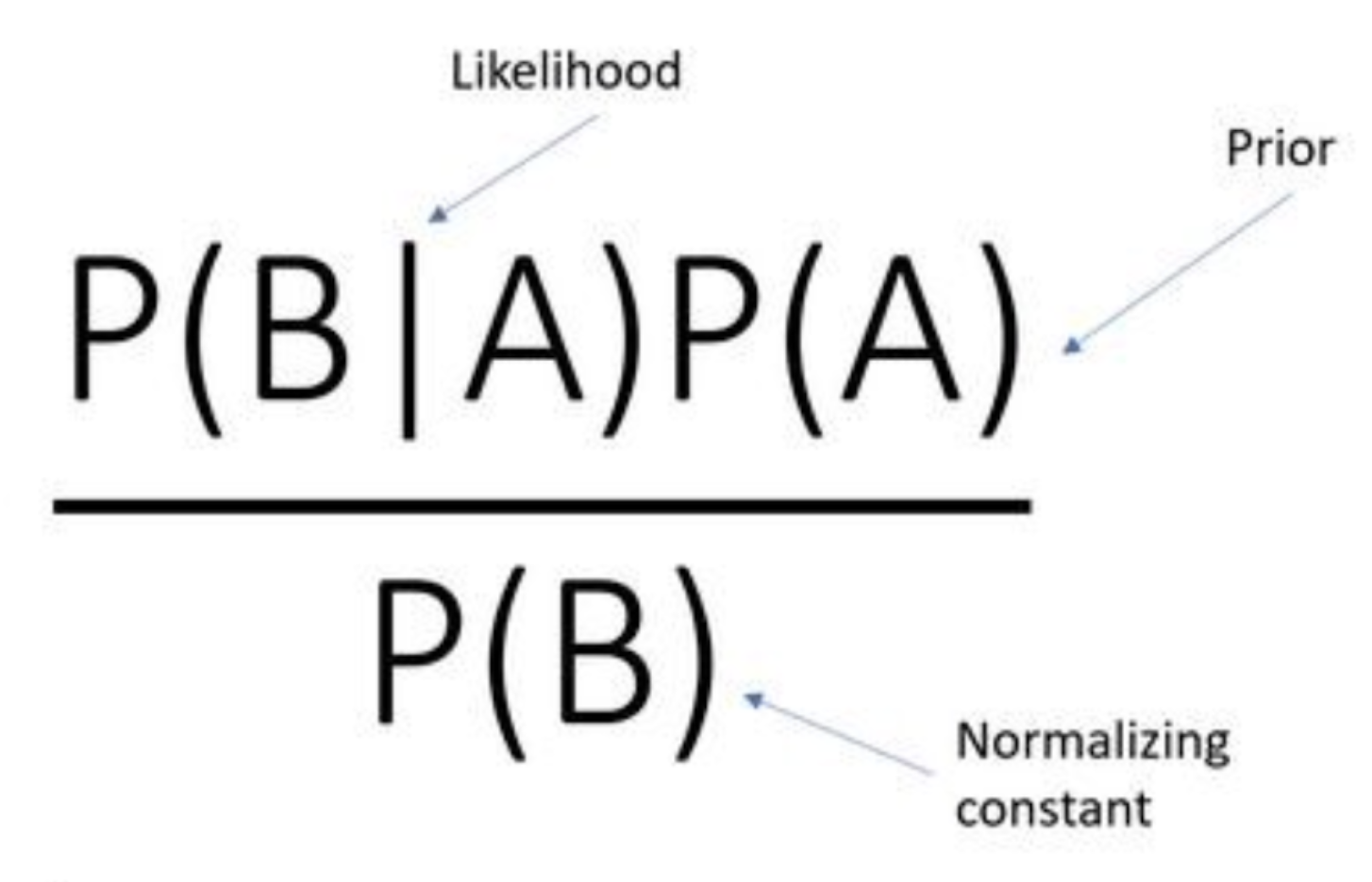
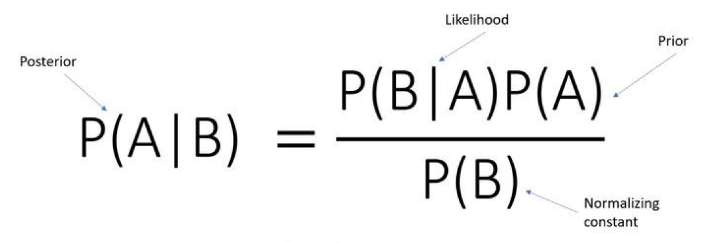
But the most interesting part in probability is the Bayes’ theorem. Since our high school, we have been encountering this theorem in many different places. Here’s the formula:
We typically get past this formula by simply feeding in the numbers and calculating the answers. But have you ever wondered what Bayes’ theorem actually tells us, what exactly is the meaning of posterior probability? Why do we even calculate it in the first place?
Let’s consider an example (no math ahead!):

This is our friend Bob. Being his classmate, we think that he is an introvert guy who often keeps to himself. We believe that he doesn’t like making friends.
So, P(A) is called the prior. In this case, we will call it our assumption that Bob rarely likes to make new friends.
Now, he meets Ed in his college.
 Unlike Bob, Ed is a laid back guy who is eager to make new friends.
P(B) in this case is the probability that Ed is friendly. On spending the day together, Bob realises that Ed and him are like two peas in a pod. As a result, they become friends.
Them becoming friends represents P(B|A):

Now, looking at the right-hand side and the example we established above, the numerator represents the probability that Bob was friendly P(A) and befriends Ed P(B|A). And all these values compute towards the result on the left-hand side, which is:
Perfect! This is exactly what we did in school, right? I’ll stretch this a little further and ask you – what does this new value mean?
Most people who claim they know Bayes’ theorem would invariably get stuck here.
This new value is nothing but our belief about Bob. Or in other words, this is our new belief about Bob and the new value of P(A).
If I were to extract the nectar of this example, it would be something like this:
We made an assumption about Bob and the evidence we found was that he actually made a new friend!
So what do we do in this case? We change our assumption about Bob, – he is not that much of an introvert. And if we happen to keep observing Bob for a few more iterations, we will eventually understand the true nature of Bob quite well.
I know what you are thinking – this looks like something we do in gradient descent and many other optimisation algorithms. We assume some random parameters, observe predictions and true values, and then readjust the parameters accordingly.
The Naive Bayes algorithm works on a similar principle, with a simple assumption that all the input features are independent. To observe this phenomenon in its full glory, we will need to dive into Bayesian networks or Probabilistic Graphical Models. They can be very powerful in their own respect and I might explore them in a future article.
Here are a couple of resources to learn more about probability:
Short MIT-OCW playlist on Probability:
Khan Academy:
Statistics for Machine Learning
This will be among the more familiar topics we’ve covered in this article. Statistics forms the backbone of machine learning and hence I have covered it here.
Whenever we talk about statistics, there are a few familiar concepts that pop into our heads:
- Measures of central tendency
- Spread of the data
- Distributions
- Hypothesis testing, etc.
Most of these concepts are fairly rudimentary. Except the last one, I have seen seasoned machine learning professionals carry around wrong intuitions about things like p-value and alpha value. Most of these play a significant role in the performance of our machine learning models like linear and logistic regression.
I know what you might be wondering – who uses linear models these days?
Well, most organisations highly favour interpretability of models ahead of accuracy. Ensemble models tend to lack that interpretability as they tend to be more biased towards performance and are extensively used in data science competitions (and not in the industry).
I’ll be honest – I was among the enthusiasts who were drawn to the fancy algorithms and preferred jumping straight to them. As a result, my predictive models yielded sub par results.
Machine learning is not just about building predictive models, but extracting as much information as possible from the given data by the statistical tools available to us.
You should check out the utterly comprehensive Applied Machine Learning course which has an entire module dedicated to statistics.
End Notes
Mathematics for machine learning is an essential facet that is often overlooked or approached with the wrong perspective. In this article, we discussed the differences between the mathematics required for data science and machine learning. We also learned some pointers on why and where we require mathematics in this field.
Please note that all the sources I mentioned for learning are not exhaustive. There are plenty of them out there and here are a couple I’ll re-iterate:


Here is another intuition for the Bayes Theorem: First, let's multiply the formula by P(B): P(A|B)*P(B) = P(B|A)*P(A) Now, let's try to interpret this equation instead. Let's go to the left side: P(B) means the probability that B happens. P(A|B) means the probability that A happens IF b happens. So, if he multiply them, we get the probability that BOTH A and B are happening at the same time! Now, let's go to the right hand side; P(A) A happens P(B|A) B happens if A happens Again, if we multiply them we get the probability that BOTH A and B are happening at the same time! We see that we deduct the same thing for both of them, so we can say that they are equivalent! How can we write that mathematically? P(A|B)*P(B) = P(B|A)*P(A) and we are done!
You did the same thing as you accused other data scientists doing. You said we need math and linked out to non relevant run or the mill math teachings with no relate-able link back to ML
Hello Kevin, If you would notice, I have provided two options in every section. One of them is very extensive and the other one is on the intuitive level. As we all know, There is no perfect content on Mathematics out there. What I pointed out is that we should ponder upon how the mathematical principle works, which I believe is available in the links I have provided. *You may choose to skip the Redundant part* Here are some Pure Intuition Resources For Linear Algebra Intuition: https://www.youtube.com/playlist?list=PLZnyIsit9AM7acLo1abCA1STjZ41ffwaM https://youtu.be/fNk_zzaMoSs For Calculus: https://youtu.be/bCx6UuzXPA0 For Probability and Statistics: https://www.youtube.com/user/jbstatistics/playlists https://www.youtube.com/playlist?list=PLORimFt-MPoxuRt8gR9rjmVKJqsJky-kf
thank you sir
Superb analysis. Where can I obtain a copy for my engineering class? Professor Plumb
Please elaborate, what exactly are you looking for?
Great article, complete, informative article. would love to follow the path. Thanks.