Introduction
Statistical analysis is a key tool for making sense of data and drawing meaningful conclusions. The chi-square test is a statistical method commonly used in data analysis to determine if there is a significant association between two categorical variables. By comparing observed frequencies to expected frequencies, the chi-square test can determine if there is a significant relationship between the variables. So let’s dive into the article to understand all about the chi-square test, what it is, how it works, and how we can implement it in R and how to calculate chi square and chi squared test.
Learning Objectives
- Understand what the chi-square test is and how it works
- Be able to calculate the chi-square value using the chi-square formula
- Learn about the different types of Chi-Square tests and where and when you should apply them
- Learn to implement a chi-square test in R
Table of contents
- What is Chi-Sqaure Test?
- When to Use the Chi-Square Test?
- Chi-Square Test Forumla
- What are Categorical Variables?
- Why Do We Use It? [Explained with Example]
- Assumptions of the Chi-Square Test
- Types of Chi-Square Tests
- Chi-Square Goodness of Fit Test
- How to Calculate Chi-Square?
- The Chi-Square Goodness of Fit Test in R
- Chi-Square Test of Association
- Chi-Square Test for Independence in R
- Limitations of Chi Square Test
- Frequently Asked Questions
What is Chi-Sqaure Test?
The chi-square test is a statistical test used to determine if there is a significant association between two categorical variables. It is a non-parametric test, meaning it does not make assumptions about the underlying distribution of the data.
It compares the observed frequencies of the categories in a contingency table with the expected frequencies that would occur under the assumption of independence between the variables. The test calculates a chi-square statistic, which measures the discrepancy between the observed and expected frequencies. We recommend these courses to readers who want to explore the topic in depth –
When to Use the Chi-Square Test?
Let’s start with a case study. I want you to think of your favorite restaurant right now. Let’s say you can predict a certain number of people arriving for lunch five days a week. At the end of the week, you observe that the expected footfall was different from the actual footfall.
Sounds like a prime statistics problem? That’s the idea!
So, how will you check the statistical significance between the observed and the expected footfall values? Remember this is a categorical variable – ‘Days of the week’ – with 5 categories [Monday, Tuesday, Wednesday, Thursday, Friday].
One of the best ways to deal with this is by using the Chi-Square test.
We can always opt for z-tests, t-tests, or ANOVA when we’re dealing with continuous variables. But the situation becomes tricky when working with categorical features (as most data scientists will attest to!). I’ve found the chi-square test to be quite helpful in my own projects.
Chi-Square Test Forumla
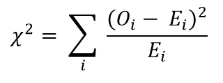
where,
- χ 2 = Chi-Square value
- Oi = Observed frequency
- Ei = Expected frequency
What are Categorical Variables?
I’m sure you’ve encountered categorial variables before, even if you might not have intuitively recognized them. They can be tricky to deal with in the data science world, so let’s first define them.
Categorical variables fall into a particular category of those variables that can be divided into finite categories. These categories are generally names or labels. These variables are also called qualitative variables as they depict the quality or characteristics of that particular variable.
For example, the category “Movie Genre” in a list of movies could contain the categorical variables – “Action”, “Fantasy”, “Comedy”, “Romance”, etc.
There are broadly two types of categorical variables:
- Nominal Variable: A nominal variable has no natural ordering to its categories. They have two or more categories. For example, Marital Status (Single, Married, Divorcee), Gender (Male, Female, Transgender), etc.
- Ordinal Variable: A variable for which the categories can be placed in an order. For example, Customer Satisfaction (Excellent, Very Good, Good, Average, Bad), and so on
When the data we want to analyze contains this type of variable, we turn to the chi-square test, denoted by χ², to test our hypothesis.
Why Do We Use It? [Explained with Example]
Let’s learn the use of chi-square with an intuitive example.
Problem Statement
A research scholar is interested in the relationship between the placement of students in the statistics department of a reputed University and their C.G.P.A (their final assessment score).
He obtains the placement records of the past five years from the placement cell database (at random). He records how many students who got placed fell into each of the following C.G.P.A. categories – 9-10, 8-9, 7-8, 6-7, and below 6.
Suppose there is no relationship between the placement rate and the C.G.P.A.. In that case, the placed students should be equally spread across the different C.G.P.A. categories (i.e., there should be similar numbers of placed students in each category).
However, if students having C.G.P.A more than 8 are more likely to get placed, then there would be a large number of placed students in the higher C.G.P.A. categories as compared to the lower C.G.P.A. categories. In this case, the data collected would make up the observed frequencies.
So the question is, are these frequencies being observed by chance, or do they follow some pattern?

Chi Square Test Solution
Here enters the chi-square test! The chi-square test helps us answer the above question by comparing the observed frequencies to the frequencies that we might expect to obtain purely by chance.
Chi-square test in hypothesis testing is used to test the hypothesis about the chi-square distribution of observations/frequencies in different categories.
We are almost at the implementing aspect of chi-square tests, but there’s one more thing we need to learn before we get there. In order to fully understand the distribution of a variable, both descriptive statistics and a chi-square test are essential tools. Descriptive statistics provide a snapshot of the data, while a chi-square test can reveal important relationships between categorical variables.
The normal distribution is a fundamental concept in statistics and is often used to model variables in experiments. A chi-square test can be used to determine if a set of observations follows a normal distribution.
Properties of Chi-Square Test
The chi-square test possesses several important properties that make it a valuable statistical tool:
| Aspect | Description |
|---|---|
| Non-parametric Test | The chi-square test is non-parametric, making no assumptions about the data’s underlying distribution. Applicable to categorical data. |
| Test for Independence | Examines association between categorical variables, determining significance of relationship or dependency, not strength or direction. |
| Goodness of Fit Test | Assesses how well observed data fit an expected distribution, comparing observed frequencies to expected frequencies. |
| Chi-Square Statistic | Measures discrepancy between observed and expected frequencies in a contingency table, indicating association or goodness of fit. |
| Degrees of Freedom | Depend on the number of categories in variables. Determine critical values and influence test result interpretation. |
| Null and Alternative Hypotheses | Null hypothesis assumes no association or difference, alternative hypothesis suggests presence of association or difference. |
| Test Statistic and P-value | Produces test statistic and corresponding p-value. Compare test statistic to critical value, p-value indicates probability under null hypothesis. |
| Interpretation | Null hypothesis rejected if test statistic exceeds critical value or p-value is less than chosen significance level. Indicates significant association or deviation. |
Assumptions of the Chi-Square Test
The chi-square test uses the sampling distribution to calculate the likelihood of obtaining the observed results by chance and to determine whether the observed and expected frequencies are significantly different. Just like any other statistical test, the chi-square test comes with a few assumptions of its own:
- A large sample size is crucial for a reliable outcome in a chi-square test, as it helps ensure that the data distribution is representative of the population.
- The χ2 assumes that the data for the study is obtained through random selection, i.e., they are randomly picked from the population.
- The categories are mutually exclusive, i.e., each subject fits into only one category. For e.g., from our above example – the number of people who lunched in your restaurant on Monday can’t be filled in the Tuesday category.
- The data should be in the form of frequencies or counts of a particular category and not in percentages.
- The data should not consist of paired samples or groups, or we can say the observations should be independent of each other.
- When more than 20% of the expected counts (frequencies) have a value of less than 5, then Chi-square cannot be used. To tackle this problem: Either one should combine the categories only if it is relevant or obtain more data.
The total number of observations is a crucial component in determining the validity of the chi-square test. The larger the number of observations, the more accurate the chi-square test results will be. The Yates correction is an adjustment used in the chi-square test to account for the expected counts (frequencies) being close to zero. The Yates correction ensures the validity of the chi-square test results when applied to small sample sizes.
Types of Chi-Square Tests
In this section, we will see the different types of chi-square tests and study them by manual calculations and with their implementation in R.
There are three main types of chi-square tests commonly used in statistics:
- Pearson’s Chi-Square Test: This test is used to determine if there is a significant association between two categorical variables in a single population. It compares the observed frequencies in a contingency table with the expected frequencies assuming independence between the variables.
- Chi-Square Goodness of Fit Test: This test is used to assess whether observed categorical data follows an expected distribution. It compares the observed frequencies with the expected frequencies specified by a hypothesized distribution.
- Chi-Square Test of Independence: This test is used to examine if there is a significant association between two categorical variables in a sample from a population. It compares the observed frequencies in a contingency table with the expected frequencies assuming independence between the variables.
Chi-Square Goodness of Fit Test
This is a non-parametric test. We typically use it to find how the observed value of a given event is significantly different from the expected value. In this case, we have categorical data for one independent variable, and we want to check whether the data distribution is similar or different from the expected distribution.
Let’s consider the above example where the research scholar was interested in the relationship between the placement of students in a reputed university’s statistics department and their C.G.P.A.
In this case, the independent variable is C.G.P.A with the categories 9-10, 8-9, 7-8, 6-7, and below 6.
The statistical question here is: whether or not the observed counts (frequencies) of placed students are equally distributed for different C.G.P.A categories (so that our theoretical frequency distribution contains the same number of students in each of the C.G.P.A categories).
We will arrange this data by using the contingency table, which will consist of both the observed and expected values as below:
| C.G.P.A | 10-9 | 9-8 | 8-7 | 7-6 | Below 6 | Total |
| Observed Frequency of Placed students | 30 | 35 | 20 | 10 | 5 | 100 |
| Expected Frequency of Placed students | 20 | 20 | 20 | 20 | 20 | 100 |
After constructing the contingency table, the next task is to compute the value of the chi-square statistic. The chi square formula is given as:
where,
- χ 2 = Chi-Square value
- Oi = Observed frequency
- Ei = Expected frequency
How to Calculate Chi-Square?
Let us look at the step-by-step approach to calculate the chi-square value
Step 1: Subtract each expected frequency from the related observed frequency
For example, for the C.G.P.A category 10-9, it will be “30-20 = 10”. Apply similar operations for all the categories.
Step 2: Square each value obtained in step 1, i.e. (O-E)2
For example: for the C.G.P.A category 10-9, the value obtained in step 1 is 10. It becomes 100 on squaring. Apply similar operations for all the categories.
Step 3: Divide all the values obtained in step 2 by the related expected frequencies, i.e. (O-E)2/E
For example: for the C.G.P.A category 10-9, the value obtained in step 2 is 100. On dividing it by the related expected frequency, which is 20, it becomes 5. Apply similar operations for all the categories.
Step 4: Add all the values obtained in step 3 to get the chi-square test statistic value
In this case, the chi-square statistic value comes out to be 32.5.
Step 5: Once we have calculated the chi-square value, we will compare it with the critical chi-square statistic value
Then the number of degrees of freedom represents the number of values in the data set that are free to vary and contribute to the test statistic. The number of degrees of freedom in the test affects the critical value and the level of significance, helping to determine if the differences are due to chance or are statistically significant. We can find the critical chi-square value in the below chi-square table against the number of degrees of freedom (number of categories – 1) and the significance level:
In this case, the degrees of freedom are 5-1 = 4. So, the critical value at a 5% significance level is 9.49. The significance level in a chi-square test determines the threshold for rejecting the null hypothesis and accepting the alternative hypothesis. A significance level of 0.05 means a 5% chance of making a Type I error or falsely rejecting the null hypothesis.
Our obtained value of 32.5 is much larger than the critical value of 9.49. Therefore, we can say that the observed frequencies from the sample data are significantly different from the expected frequencies. In other words, C.G.P.A is related to the number of placements that occur in the department of statistics.
Let’s further solidify our understanding by performing the Chi-Square test in R.
The Chi-Square Goodness of Fit Test in R
Let’s implement the chi-square goodness of fit test in R. Time to fire up RStudio!
Problem Statement
Let’s understand the problem statement before we dive into R.
An organization claims that the experience of the employees of different departments is distributed in the following categories:
- 11 – 20 Years = 20%
- 21 – 40 Years = 17%
- 6 – 10 Years = 41% and
- Up to 5 Years = 22%
A random sample of 1470 employees is collected. Does this random sample provide evidence against the organization’s claim?
You can download the data here.
Setting up the Hypothesis
- Null hypothesis: The true proportions of the experience of the employees of different departments are distributed in the following categories: 11 – 20 Years = 20%, 21 – 40 Years = 17%, 6 – 10 Years = 41%, and up to 5 Years = 22%
- Alternative hypothesis: The distribution of experience of the employees of different departments differs from what the organization states
Let’s begin!
Step 1: First, import the data
Step 2: Validate it for correctness in R
Output:
 #Count of Rows and columns

[1] 1470 2
#View top 10 rows of the dataset

age.intervals Experience.intervals
1 41 - 50 6 - 10 Years
2 41 - 50 6 - 10 Years
3 31 - 40 6 - 10 Years
4 31 - 40 6 - 10 Years
5 18 - 30 6 - 10 Years
6 31 - 40 6 - 10 Years
7 51 - 60 11 - 20 Years
8 18 - 30 Upto 5 Years
9 31 - 40 6 - 10 Years
10 31 - 40 11 - 20 Years
Step 3: Create a proportion table for expected frequencies:
Output:
11 - 20 Years 21 - 40 Years 6 - 10 Years Upto 5 Years
0.2312925 0.1408163 0.4129252 0.2149660
Step – 4: Calculate the chi-square value
Output:
Chi-square test for given probabilities

data: table(data$Experience.intervals)
X-squared = 14.762, df = 3, p-value = 0.002032
The p-value here is less than 0.05. Therefore, we will reject our null hypothesis. Hence, the distribution of experience of the employees of different departments differs from what the organization states.
Chi-Square Test of Association
The second type of chi-square test is the Pearson’s chi-square test of association. This test is used when we have categorical data for two independent variables and want to see if there is any relationship between the variables.
Let’s take another example to understand this. A teacher wants to know whether the outcome of a mathematics test is related to the gender of the person taking the test. Or in other words, she wants to know if males show a different pattern of pass/fail rates than females.
So, here are two categorical variables: Gender (Male and Female) and mathematics test outcome (Pass or Fail). Let us now look at the contingency table:
| Status | Boys | Girls |
| Pass | 17 | 20 |
| Fail | 8 | 5 |
Looking at the above contingency table, we can see that girls have a comparatively higher pass rate than boys. However, to test whether or not this observed difference is significant, we will carry out the chi-square test.
The steps to calculate the chi square test value are as follows:
Step 1: Calculate the row and column total of the above contingency table
| Status | Boys | Girls | Total |
| Pass | 17 | 20 | 37 |
| Fail | 8 | 5 | 13 |
| Total | 25 | 25 | 50 |
Step 2: Calculate the expected frequency for each individual cell by multiplying row sum by column sum and dividing by total number
Expected Frequency = (Row Total x Column Total)/Grand Total
For the first cell, the expected frequency would be (37*25)/50 = 18.5. Now, write them below the observed frequencies in brackets:
| Status | Boys | Girls | Total |
| Pass | 17 (18.5) | 20 (18.5) | 37 |
| Fail | 8 | 5 | 13 |
| Total | 25 | 25 | 50 |
Step 3: Calculate the value of chi-square using the formula
Calculate the right-hand side part of each cell. For example, for the first cell, ((17-18.5)^2)/18.5 = 0.1216.
Step 4: Then, add all the values obtained for each cell. In this case, the values are
0.1216+0.1216+0.3461+0.3461 = 0.9354
Step 5: Calculate the degrees of freedom, i.e (Number of rows-1)*(Number of columns-1) = 1*1 = 1
The next task is to compare it with the critical chi-square value from the above table.
The Chi-Square calculated value is 0.9354, which is less than the critical value of 3.84. So, in this case, we fail to reject the null hypothesis. This means there is no significant association between the two variables, i.e., boys and girls have a statistically similar pattern of pass/fail rates on their mathematics tests.
Let’s further solidify our understanding by performing the chi square test test in R.
Chi-Square Test for Independence in R
Problem Statement
A Human Resources department of an organization wants to check whether the employees’ age and experience depend on each other. For this purpose, a random sample of 1470 employees is collected with their age and experience. You can download the data here.
Setting up the hypothesis:
- Null hypothesis: Age and Experience are two independent variables
- Alternative hypothesis: Age and Experience are two dependent variables
Let’s begin!
Step 1: First, import the data
Step 2: Validate it for correctness in R:
Output:
 #Count of Rows and columns

[1] 1470 2
> #View top 10 rows of the dataset

age.intervals Experience.intervals
1 41 - 50 6 - 10 Years
2 41 - 50 6 - 10 Years
3 31 - 40 6 - 10 Years
4 31 - 40 6 - 10 Years
5 18 - 30 6 - 10 Years
6 31 - 40 6 - 10 Years
7 51 - 60 11 - 20 Years
8 18 - 30 Upto 5 Years
9 31 - 40 6 - 10 Years
10 31 - 40 11 - 20 Years
Step 3: Construct a contingency table and calculate the chi-square value:
Output:
ct<-table(data$age.intervals,data$Experience.intervals)
> ct

11 - 20 Years 21 - 40 Years 6 - 10 Years Upto 5 Years
18 - 30 22 0 172 192
31 - 40 190 20 308 101
41 - 50 85 112 110 15
51 - 60 43 75 17 8
> chisq.test(ct)

Pearson's Chi-squared test

data: ct
X-squared = 679.97, df = 9, p-value < 2.2e-16
The p-value here is less than 0.05. Therefore, we will reject our null hypothesis. We can conclude that age and experience are two dependent variables, aka, as the experience increases, the age also increases (and vice versa).
Limitations of Chi Square Test
While the chi-square test is a useful statistical tool, it does have some limitations that should be considered:
- Independence Assumption: The test assumes independent observations, contributing to expected frequencies. Violations like dependence or correlation can impact validity.
- Sample Size: Reliability is limited with small samples or low expected cell frequencies. Recommended to have at least 5 frequencies scheduled per cell.
- Sensitivity to Sample Composition: Imbalanced frequencies or empty cells can bias or inaccurately influence test results.
- Limited to Categorical Variables: Designed for categorical variables; not applicable to continuous or ordinal variables.
- Lack of Directionality or Magnitude: Determines association presence but doesn’t indicate strength, direction, or magnitude.
- Type of Association: Detects associations but doesn’t differentiate types or establish cause-and-effect relationships.
- Large Sample Bias: In large samples, small deviations may lead to statistically significant results without practical implications.
- Multiple Comparisons: Multiple tests on the same data increase the chance of finding significant results by chance alone. Consider adjustments like Bonferroni correction.
- Interpretation Considerations: Interpret test results cautiously, considering the context and research question. Significance doesn’t guarantee meaningful or practically important associations.
Conclusion
In this article, we learned how to analyze the significant difference between data that contains categorical measures with the help of chi-square tests. We enhanced our knowledge of the use of chi-square, the assumptions involved in carrying out the test, and how to conduct different types of chi-square tests both manually and in R.
If you are new to statistics, want to cover your basics, and also want to get a start in data science, I recommend taking the Introduction to Data Science course. It gives you a comprehensive overview of both descriptive and inferential statistics before diving into data science techniques.
Did you find this article useful? Can you think of any other applications of the chi-square test? We have covered all about the chi squared test and also what is chi square test is a test of with you will also get how to calculate chi square test. Let me know in the comments section below, and we can come up with more ideas!
Key Takeaways
- The Chi-square test is a hypothesis testing method used to compare observed data with expected data.
- The chi-square value, calculated using the chi-square formula, tells us the extent of similarity or difference between the categories of data being considered.
- There are two types of Chi-Square Tests: the Chi-Square Goodness of Fit Test and the Chi-Square Test of Independence/Association.
Frequently Asked Questions
Q1. What is the chi-square test used for?
A. The chi-square test is used to determine if there’s a significant association between two categorical variables. It helps to see if the observed frequencies (counts) of events differ from the expected frequencies if the variables were independent.
Q2.How do you interpret the results of a chi-square test?
A. To interpret the results:
Compare the p-value to a significance level (like 0.05).
If p-value is less than 0.05, there is a significant association between the variables (they are not independent).
If p-value is greater than 0.05, there is no significant association (they are independent).
Q3. What is the p-value in a chi-square test?
A. The p-value in a chi-square test indicates the probability that the observed differences occurred by chance. A lower p-value suggests that the observed differences are unlikely to have occurred by chance, implying a significant association between the variables.
Q4. What type of data is suitable for a chi-square test?
A. Data suitable for a chi-square test are categorical data, which can be divided into different categories or groups. Examples include data like gender (male/female), yes/no responses, or different age groups. The data should be in the form of counts or frequencies.


Very simple yet good explanation of Chi Square test. Thanks for the post
Loved it, very well explained.
So appreciate for this simple but powerful explanation of application of Chi Square Test. May God bless you.
The piece was very educating. Many thanks
It's amazing. I love it and easy to understand. Cheers.
It was very useful and helpful. Thank you very much.