Imagine you’re lost in a dense forest with no map or compass. What do you do? You follow the path of the steepest descent, taking steps in the direction that decreases the slope and brings you closer to your destination. Similarly, gradient descent is the go-to algorithm for navigating the complex landscape of machine learning and deep learning. It helps models find the optimal set of parameters by iteratively adjusting them in the opposite direction of the gradient. This article will deeply dive into gradient descent, exploring its different flavors, applications, and challenges. Get ready to sharpen your optimization skills and join the ranks of the machine learning elite!
In this article, We have talked about the gradient descent and what is gradient descent , how to implement gradient descent python , What is Gradient descent in machine learning these all topics we have covered . so lets start .
Learning objectives:
This article was published as a part of the Data Science Blogathon.
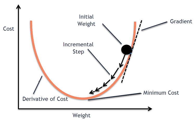
It is a function that measures the performance of a model for any given data. Cost Function quantifies the error between predicted values and expected values and presents it in the form of a single real number.
After making a hypothesis with initial parameters, we calculate the Cost function. And with a goal to reduce the cost function, we modify the parameters by using the Gradient descent algorithm over the given data. Here’s the mathematical representation for it:
_LI.jpg)
Gradient descent is an optimization algorithm used in machine learning to minimize the cost function by iteratively adjusting parameters in the direction of the negative gradient, aiming to find the optimal set of parameters.
The cost function represents the discrepancy between the predicted output of the model and the actual output. Gradient descent aims to find the parameters that minimize this discrepancy and improve the model’s performance.
The algorithm operates by calculating the gradient of the cost function, which indicates the direction and magnitude of the steepest ascent. However, since the objective is to minimize the cost function, gradient descent moves in the opposite direction of the gradient, known as the negative gradient direction.
By iteratively updating the model’s parameters in the negative gradient direction, gradient descent gradually converges towards the optimal set of parameters that yields the lowest cost. The learning rate, a hyperparameter, determines the step size taken in each iteration, influencing the speed and stability of convergence.
Gradient descent can be applied to various machine learning algorithms, including linear regression, logistic regression, neural networks, and support vector machines. It provides a general framework for optimizing models by iteratively refining their parameters based on the cost function.
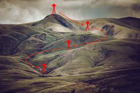
Let’s say you are playing a game in which the players are at the top of a mountain and asked to reach the lowest point of the mountain. Additionally, they are blindfolded. So, what approach do you think would make you reach the lake?
Take a moment to think about this before you read on.
The best way is to observe the ground and find where the land descends. From that position, step in the descending direction and iterate this process until we reach the lowest point.
Finding the lowest point in a hilly landscape.
Gradient descent is an iterative optimization algorithm for finding the local minimum of a function.
To find the local minimum of a function using gradient descent, we must take steps proportional to the negative of the gradient (move away from the gradient) of the function at the current point. If we take steps proportional to the positive of the gradient (moving towards the gradient), we will approach a local maximum of the function, and the procedure is called Gradient Ascent.
Gradient descent was originally proposed by CAUCHY in 1847. It is also known as the steepest descent.
The goal of the gradient descent algorithm is to minimize the given function (say, cost function). To achieve this goal, it performs two steps iteratively:

Alpha is called Learning rate – a tuning parameter in the optimization process. It decides the length of the steps.
Here how you can implement gradient descent Python:
import numpy as np

def gradient_descent(X, y, learning_rate, num_iters):
  """
  Performs gradient descent to find optimal weights and bias for linear regression.

  Args:
      X: A numpy array of shape (m, n) representing the training data features.
      y: A numpy array of shape (m,) representing the training data target values.
      learning_rate: The learning rate to control the step size during updates.
      num_iters: The number of iterations to perform gradient descent.

  Returns:
      A tuple containing the learned weights and bias.
  """

  # Initialize weights and bias with random values
  m, n = X.shape
  weights = np.random.rand(n)
  bias = 0

  # Loop for the number of iterations
  for i in range(num_iters):
    # Predict y values using current weights and bias
    y_predicted = np.dot(X, weights) + bias

    # Calculate the error
    error = y - y_predicted

    # Calculate gradients for weights and bias
    weights_gradient = -2/m * np.dot(X.T, error)
    bias_gradient = -2/m * np.sum(error)

    # Update weights and bias using learning rate
    weights -= learning_rate * weights_gradient
    bias -= learning_rate * bias_gradient

  return weights, bias

# Example usage
X = np.array([[1, 1], [2, 2], [3, 3]])
y = np.array([2, 4, 5])
learning_rate = 0.01
num_iters = 100

weights, bias = gradient_descent(X, y, learning_rate, num_iters)

print("Learned weights:", weights)
print("Learned bias:", bias)
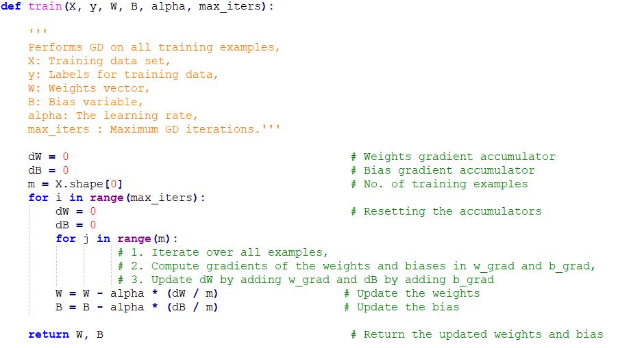
This code creates a function called gradient_descent, which requires the training data, learning rate, and number of iterations as parameters. It carries out the Number of Steps :
1.Sets weights and bias to arbitrary values during initialization.
2.Executes a set number of iterations for loops.
3.Computes the estimated y values by utilizing the existing weights and bias.
4.Calculates the discrepancy between expected and real y values.
5.Determines the changes in the cost function based on weights and bias.
6.Adjusts the weights and bias by incorporating the gradients and learning rate.
7.Outputs the acquired weights and bias.
The choice of gradient descent algorithm depends on the problem at hand and the size of the dataset. Batch gradient descent is suitable for small datasets, while stochastic gradient descent algorithm is more suitable for large datasets. Mini-batch is a good compromise between the two and is often used in practice.
Batch gradient descent updates the model’s parameters using the gradient of the entire training set. It calculates the average gradient of the cost function for all the training examples and updates the parameters in the opposite direction. Batch gradient descent guarantees convergence to the global minimum but can be computationally expensive and slow for large datasets.
Stochastic gradient descent updates the model’s parameters using the gradient of one training example at a time. It randomly selects a training dataset example, computes the gradient of the cost function for that example, and updates the parameters in the opposite direction. Stochastic gradient descent is computationally efficient and can converge faster than batch gradient descent. However, it can be noisy and may not converge to the global minimum.
Mini-batch gradient descent updates the model’s parameters using the gradient of a small batch size of the training dataset, known as a mini-batch. It calculates the average gradient of the cost function for the mini-batch and updates the parameters in the opposite direction. The mini-batch gradient descent algorithm combines the advantages of batch and stochastic gradient descent. It is the most commonly used method in practice. It is computationally efficient and less noisy than stochastic gradient descent while still being able to converge to a good solution.
When we have a single parameter (theta), we can plot the dependent variable cost on the y-axis and theta on the x-axis. If there are two parameters, we can go with a 3-D plot, with cost on one axis and the two parameters (thetas) along the other two axes.

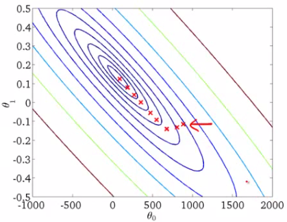
It can also be visualized by using Contours. This shows a 3-D plot in two dimensions with parameters along axes and the response as a contour. The value of the response increases away from the center and has the same value as with the rings. The response is directly proportional to the distance of a point from the center (along a direction).
We have the direction we want to move in. Now, we must decide the size of the step we must take.
*It must be chosen carefully to end up with local minima.
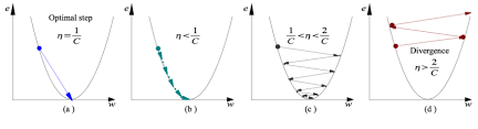
Note: As the gradient decreases while moving towards the local minima, the size of the step decreases. So, the learning rate (alpha) can be constant over the optimization and need not be varied iteratively.
The cost function may consist of many minimum points. Depending on the initial point (i.e., initial parameters(theta)) and the learning rate, the gradient may settle on any minima. Therefore, the optimization may converge to different starting points and learning rates.
Easy to use: It’s like rolling the marble yourself – no fancy tools needed, you just gotta push it in the right direction.
Fast updates: Each push (iteration) is quick, you don’t have to spend a lot of time figuring out how hard to push.
Memory efficient: You don’t need a big backpack to carry around extra information, just the marble and your knowledge of the hill.
Usually finds a good spot: Most of the time, the marble will end up in a pretty flat area, even if it’s not the absolute flattest (global minimum).
Slow for giant hills (large datasets): If the hill is enormous, pushing the marble all the way down each time can be super slow. There are better ways to roll for these giants.
Can get stuck in shallow dips (local minima): The hill might have many dips, and the marble could get stuck in one that isn’t the absolute lowest. It depends on where you start pushing it from.
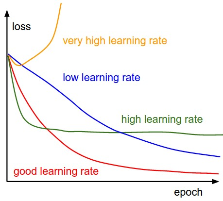
Finding the perfect push (learning rate): You need to figure out how har to push the marble (learning rate). If you push too weakly, it’ll take forever to get anywhere. Push too hard, and it might roll right past the flat spot.
While gradient descent is a powerful optimization algorithm, it can also present some challenges affecting its performance. Some of these challenges include:
Researchers have developed several variations of gradient descent algorithms to overcome these challenges, such as adaptive learning rate, momentum-based, and second-order methods. Additionally, choosing the right regularization method, model architecture, and hyperparameters can also help improve the performance of the gradient descent algorithm.
In conclusion, the gradient descent algorithm is a cornerstone of machine learning optimization techniques. Much like finding your way out of a dense forest by following the path of the steepest descent, gradient descent guides ML models toward optimal performance by iteratively adjusting parameters to minimize the cost function. This method’s effectiveness in navigating the complex landscape of model training is unparalleled. Whether applied to linear regression model, neural networks, or deep learning frameworks.
Hope you like the article , So We have Covered this topics Which many of you given suggestions to covered :
By mastering gradient descent, you equip yourself with a powerful tool to enhance machine learning models, making them more accurate and reliable. Whether working with small datasets or scaling up to deep learning applications, understanding and effectively implementing gradient descent will significantly elevate your optimization and machine learning expertise. As you continue to explore and refine these techniques, you are poised to make substantial contributions to the ever-evolving field of data science.
If you want to enhance your skills in gradient descent and other advanced topics in machine learning, check out the Analytics Vidhya AI & ML Blackbelt program. This program provides comprehensive training and hands-on experience with the latest tools and techniques used in data science, including gradient descent, artificial intelligence, natural language processing, deep learning, machine learning, and more. By enrolling in this program, you can gain the knowledge and skills needed to advance your career in data science and become a highly sought-after professional in this fast-growing field. Take the first step towards your data science career today!
A. A gradient-based algorithm is an optimization method that uses the gradient of the objective function to find the function’s minimum or maximum. In machine learning, these algorithms iteratively adjust the model parameters in a direction that reduces the error by computing the gradient of the loss function for the parameters.
A. The “best” gradient descent algorithm depends on the specific problem and context. But Adam (Adaptive Moment Estimation) is widely regarded as one of the most effective and popular algorithms. This is due to its adaptive learning rate and momentum, which help to accelerate convergence and improve performance on a wide range of tasks.
A. There are three types of gradient descent: batch gradient descent, stochastic gradient descent, and mini-batch gradient descent. These methods differ in updating the model’s parameters and the size of the data batches used in each iteration.
A. Gradient descent is an optimization algorithm that minimizes the cost function in linear regression. It iteratively updates the model’s parameters by computing the partial derivatives of the cost function concerning each parameter and adjusting them in the opposite direction of the gradient.
A. SGD is usually faster than batch gradient descent, especially for large datasets. But it can be noisier. Mini-batch give a good balance between speed and stability.
Lorem ipsum dolor sit amet, consectetur adipiscing elit,


