Introduction
Understanding this network helps us to obtain information about the underlying reasons in the advanced models of Deep Learning. Multilayer Perceptron is commonly used in simple regression problems. However, MLPs are not ideal for processing patterns with sequential and multidimensional data.
🙄 A multilayer perceptron strives to remember patterns in sequential data, because of this, it requires a “large” number of parameters to process multidimensional data.
For sequential data, the RNNs are the darlings because their patterns allow the network to discover dependence 🧠 on the historical data, which is very useful for predictions. For data, such as images and videos, CNNs excel at extracting resource maps for classification, segmentation, among other tasks.
In some cases, a CNN in the form of Conv1D / 1D is also used for networks with sequential input data. However, in most models of Deep Learning, MLP, CNN, or RNN are combined to make the most of each.
MLP, CNN, and RNN don’t do everything…
Much of its success comes from identifying its objective and the good choice of some parameters, such as Loss function, Optimizer, and Regularizer.
We also have data from outside the training environment. The role of the Regularizer is to ensure that the trained model generalizes to new data.
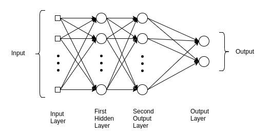
Table of contents
This article was published as a part of the Data Science Blogathon.
Dataset MNIST
Suppose our goal is to create a network to identify numbers based on handwritten digits. For example, when the entrance to the network is an image of a number 8, the corresponding forecast must also be 8.
🤷🏻♂️ This is a basic job of classification with neural networks.
The National Institute of Standards and Technology dataset, or MNIST, is considered as the Hello World! Deep Learning datasets.
Before dissecting the MLP model, it is essential to understand the MNIST dataset. It is used to explain and validate many theories of deep learning because the 70,000 images it contains are small but sufficiently rich in information;

MNIST is a collection of digits ranging from 0 to 9. It has a training set of 60,000 images and 10,000 tests classified into categories.
To use the MNIST dataset in TensorFlow is simple.
import numpy as np
from tensorflow.keras.datasets import mnist
(x_train, y_train), (x_test, y_test) = mnist.load_data()
The mnist.load_data() method is convenient, as there is no need to load all 70,000 images and their labels.
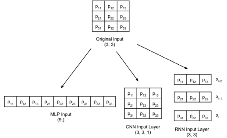
Before entering the Multilayer Perceptron classifier, it is essential to keep in mind that, although the MNIST data consists of two-dimensional tensors, they must be remodeled, depending on the type of input layer.
A 3×3 grayscale image is reshaped for the MLP, CNN and RNN input layers:
The labels are in the form of digits, from 0 to 9.
num_labels = len(np.unique(y_train))
print("total de labels:t{}".format(num_labels))
print("labels:ttt{0}".format(np.unique(y_train)))
⚠️ This representation is not suitable for the forecast layer that generates probability by class. The most suitable format is one-hot, a 10-dimensional vector-like all 0 values, except the class index. For example, if the label is 4, the equivalent vector is [0,0,0,0, 1, 0,0,0,0,0].
In Deep Learning, data is stored in a tensor. The term tensor applies to a scalar-tensor (tensor 0D), vector (tensor 1D), matrix (two-dimensional tensor), and multidimensional tensor.
#converter em one-hot
from tensorflow.keras.utils import to_categorical
y_train = to_categorical(y_train)
y_test = to_categorical(y_test)
Our model is an MLP, so your inputs must be a 1D tensor. as such, x_train and x_test must be transformed into [60,000, 2828] and [10,000, 2828],
In numpy, the size of -1 means allowing the library to calculate the correct dimension. In the case of x_train, it is 60,000.
image_size = x_train.shape[1]
input_size = image_size * image_size

print("x_train:t{}".format(x_train.shape))
print("x_test:tt{}n".format(x_test.shape))

x_train = np.reshape(x_train, [-1, input_size])
x_train = x_train.astype('float32') / 255

x_test = np.reshape(x_test, [-1, input_size])
x_test = x_test.astype('float32') / 255

print("x_train:t{}".format(x_train.shape))
print("x_test:tt{}".format(x_test.shape))
Output:
x_train:	(60000, 28, 28)
x_test:		(10000, 28, 28)

x_train:	(60000, 784)
x_test:		(10000, 784)
Building the model

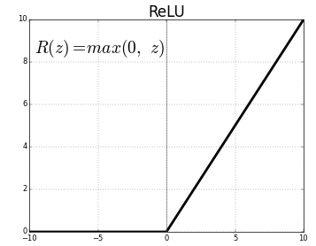
Our model consists of three Multilayer Perceptron layers in a Dense layer. The first and second are identical, followed by a Rectified Linear Unit (ReLU) and Dropout activation function.
from tensorflow.keras.models import Sequential
from tensorflow.keras.layers import Dense, Activation, Dropout

# Parameters
batch_size = 128 # It is the sample size of inputs to be processed at each training stage.
hidden_units = 256
dropout = 0.45

# Nossa  MLP com ReLU e Dropout
model = Sequential()

model.add(Dense(hidden_units, input_dim=input_size))
model.add(Activation('relu'))
model.add(Dropout(dropout))

model.add(Dense(hidden_units))
model.add(Activation('relu'))
model.add(Dropout(dropout))

model.add(Dense(num_labels))
Regularization
A neural network has a tendency to memorize its training data, especially if it contains more than enough capacity. In this case, the network fails catastrophically when subjected to the test data.
This is the classic case that the network fails to generalize (Overfitting / Underfitting). To avoid this trend, the model uses a regulatory layer. Dropout.
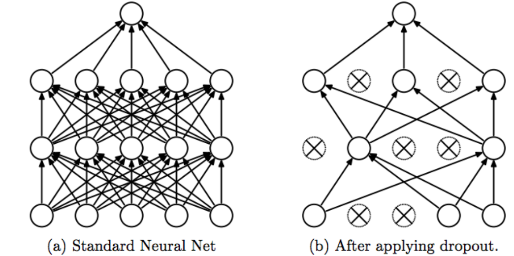
The idea of Dropout is simple. Given a discard rate (in our model, we set = 0.45) the layer randomly removes this fraction of units.
For example, if the first layer has 256 units, after Dropout (0.45) is applied, only (1 – 0.45) * 255 = 140 units will participate in the next layer
Dropout makes neural networks more robust for unforeseen input data, because the network is trained to predict correctly, even if some units are absent.
⚠️ Dropout only participates in “play” 🤷🏻♂️ during training.
Activation
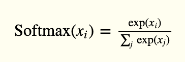
The output layer has 10 units, followed by a softmax activation function. The 10 units correspond to the 10 possible labels, classes or categories.
The activation of softmax can be expressed mathematically, according to the following equation:
model.add(Activation('softmax'))
model.summary()
Output:
Model: "sequential"
_________________________________________________________________
Layer (type)                 Output Shape              Param #
=================================================================
dense (Dense)                (None, 256)               200960
_________________________________________________________________
activation (Activation)      (None, 256)               0
_________________________________________________________________
dropout (Dropout)            (None, 256)               0
_________________________________________________________________
dense_1 (Dense)              (None, 256)               65792
_________________________________________________________________
activation_1 (Activation)    (None, 256)               0
_________________________________________________________________
dropout_1 (Dropout)          (None, 256)               0
_________________________________________________________________
dense_2 (Dense)              (None, 10)                2570
_________________________________________________________________
activation_2 (Activation)    (None, 10)                0
=================================================================
Total params: 269,322
Trainable params: 269,322
Non-trainable params: 0
_________________________________________________________________
Model Visualization Optimization
The purpose of Optimization is to minimize the loss function. The idea is that if the loss is reduced to an acceptable level, the model indirectly learned the function that maps the inputs to the outputs. Performance metrics are used to determine whether your model has learned.
model.compile(loss='categorical_crossentropy', optimizer='adam', metrics=['accuracy'])- Categorical_crossentropy, is used for one-hot
- Accuracy is a good metric for classification tasks.
- Adam is an optimization algorithm that can be used instead of the classic stochastic gradient descent procedure
📌 Given our training set, the choice of loss function, optimizer and regularizer, we can start training our model.
model.fit(x_train, y_train, epochs=20, batch_size=batch_size)OUTPUT:
Epoch 1/20
469/469 [==============================] - 1s 3ms/step - loss: 0.4230 - accuracy: 0.8690

....

Epoch 20/20
469/469 [==============================] - 2s 4ms/step - loss: 0.0515 - accuracy: 0.9835
Evaluation
At this point, our MNIST digit classifier model is complete. Your performance evaluation will be the next step in determining whether the trained model will present a sub-optimal solution
_, acc = model.evaluate(x_test,
                        y_test,
                        batch_size=batch_size,
                        verbose=0)
print("nAccuracy: %.1f%%n" % (100.0 * acc))
Output:
Accuracy: 98.4%Frequently Asked Questions
Q1. What is MLP in simple terms?
A. In simple terms, MLP, or Multilayer Perceptron, is a type of artificial neural network designed to learn complex patterns and relationships, mimicking human brain functionality.
Q2. What is the theory of multilayer perceptron?
A. The theory of multilayer perceptron involves interconnected layers of artificial neurons, each layer processing information and contributing to the network’s ability to understand intricate patterns in data.
Q3. How does an MLP work?
A. An MLP works by passing input data through multiple layers of interconnected neurons, each layer transforming the input, learning features, and contributing to the network’s ability to make accurate predictions or classifications.
Q4. What is the architecture of the Multilayer Perceptron (MLP) network?
A. The architecture of an MLP network comprises an input layer, one or more hidden layers, and an output layer. Neurons in each layer are interconnected, and the network learns by adjusting weights during training.


