Cost Function is No Rocket Science!
Introduction
In this article, we’ll talk about cost functions in machine learning. We’ll discuss why they’re important and how they help evaluate how well a model performs. We’ll also look at different types of cost functions used for predicting continuous values and categories.
This article was published as a part of the Data Science Blogathon.

The 2 main questions that popped up in my mind while working on this article were “Why am I writing this article?” & “How is my article different from other articles?” Well, the cost function is an important concept to understand in the fields of data science but while pursuing my post-graduation, I realized that the resources available online are too general and didn’t address my needs completely.
I had to refer to many articles & see some videos on YouTube to get an intuition behind cost functions. As a result, I wanted to put together the “What,” “When,” “How,” and “Why” of Cost functions that can help to explain this topic more clearly. I hope that my article acts as a one-stop-shop for cost functions!
Table of contents
What is Cost Function ?
A cost function, also referred to as a loss function or objective function, is a key concept in machine learning. It quantifies the difference between predicted and actual values, serving as a metric to evaluate the performance of a model. The primary objective is to minimize the cost function, indicating better alignment between predicted and observed outcomes. In essence, the cost function in machine learning guides the model towards optimal predictions by measuring its accuracy against the training data.
Loss function: Used when we refer to the error for a single training example.
Cost function: Used to refer to an average of the loss functions over an entire training dataset.
Why to use a Cost function?
Why on earth do we need a cost function? Consider a scenario where we wish to classify data. Suppose we have the height & weight details of some cats & dogs. Let us use these 2 features to classify them correctly. If we plot these records, we get the following scatterplot:
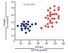
Blue dots are cats & red dots are dogs. Following are some solutions to the above classification problem.
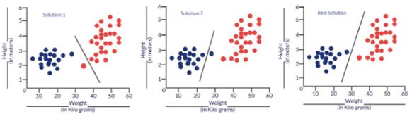
Essentially all three classifiers have very high accuracy but the third solution is the best because it does not misclassify any point. The reason why it classifies all the points perfectly is that the line is almost exactly in between the two groups, and not closer to any one of the groups. This is where the concept of cost function comes in. Cost function helps us reach the optimal solution. The cost function is the technique of evaluating “the performance of our algorithm/model”.
It takes both predicted outputs by the model and actual outputs and calculates how much wrong the model was in its prediction. It outputs a higher number if our predictions differ a lot from the actual values. As we tune our model to improve the predictions, the cost function acts as an indicator of how the model has improved. This is essentially an optimization problem. The optimization strategies always aim at “minimizing the cost function”.
What is Cost Function in Machine learning
A cost function in Machine Learning is an essential tool in machine learning for assessing the performance of a model. It basically measures the discrepancy between the model’s predictions and the true values it is attempting to predict. This variance is depicted as a lone numerical figure, enabling us to measure the model’s precision.

Here is an explanation of the function of a cost function:
Error calculation: It determines the difference between the predicted outputs (what the model predicts as the answer) and the actual outputs (the true values we possess for the data).
Gives one value: This simplifies comparing the model’s performance on various datasets or training rounds.
Improving Guides: The objective is to reduce the cost function. Through modifying the internal parameters of the model such as weights and biases, we can aim to minimize the total error and enhance the accuracy of the model.
Consider this scenario: envision yourself instructing a model to forecast the prices of houses. The cost function indicates the difference between your model’s predictions and the actual market values. By reducing this cost function, you are essentially adjusting the model to enhance its accuracy in making future predictions.
Types of Cost function in machine learning
There are many cost functions in machine learning and each has its use cases depending on whether it is a regression problem or classification problem.
- Regression cost Function
- Binary Classification cost Functions
- Multi-class Classification cost Functions
1. Regression cost Function:
Regression models deal with predicting a continuous value for example salary of an employee, price of a car, loan prediction, etc. A cost function used in the regression problem is called “Regression Cost Function”. They are calculated on the distance-based error as follows:
Error = y-y’
Where,
Y – Actual Input
Y’ – Predicted output
The most used Regression cost functions are below,
1.1 Mean Error (ME)
- In this cost function, the error for each training data is calculated and then the mean value of all these errors is derived.
- Calculating the mean of the errors is the simplest and most intuitive way possible.
- The errors can be both negative and positive. So they can cancel each other out during summation giving zero mean error for the model.
- Thus this is not a recommended cost function but it does lay the foundation for other cost functions of regression models.
1.2 Mean Squared Error (MSE)
- This improves the drawback we encountered in Mean Error above. Here a square of the difference between the actual and predicted value is calculated to avoid any possibility of negative error.
- It is measured as the average of the sum of squared differences between predictions and actual observations.
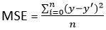
MSE = (sum of squared errors)/n
- It is also known as L2 loss.
- In MSE, since each error is squared, it helps to penalize even small deviations in prediction when compared to MAE. But if our dataset has outliers that contribute to larger prediction errors, then squaring this error further will magnify the error many times more and also lead to higher MSE error.
- Hence we can say that it is less robust to outliers
1.3 Mean Absolute Error (MAE)
- This cost function also addresses the shortcoming of mean error differently. Here an absolute difference between the actual and predicted value is calculated to avoid any possibility of negative error.
-
So in this cost function, MAE is measured as the average of the sum of absolute differences between predictions and actual observations.
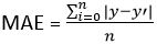
MAE = (sum of absolute errors)/n
- It is also known as L1 Loss.
- It is robust to outliers thus it will give better results even when our dataset has noise or outliers.
2. Cost functions for Classification problems
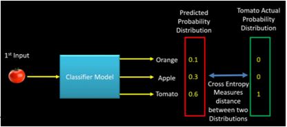
Cost functions used in classification problems are different than what we use in the regression problem. A commonly used loss function for classification is the cross-entropy loss. Let us understand cross-entropy with a small example. Consider that we have a classification problem of 3 classes as follows.
Class(Orange,Apple,Tomato)
The machine learning model will give a probability distribution of these 3 classes as output for a given input data. The class with the highest probability is considered as a winner class for prediction.
Output = [P(Orange),P(Apple),P(Tomato)]
The actual probability distribution for each class is shown below.
Orange = [1,0,0]
Apple = [0,1,0]
Tomato = [0,0,1]
If during the training phase, the input class is Tomato, the predicted probability distribution should tend towards the actual probability distribution of Tomato. If the predicted probability distribution is not closer to the actual one, the model has to adjust its weight. This is where cross-entropy becomes a tool to calculate how much far the predicted probability distribution from the actual one is. In other words, Cross-entropy can be considered as a way to measure the distance between two probability distributions. The following image illustrates the intuition behind cross-entropy:
This was just an intuition behind cross-entropy. It has its origin in information theory. Now with this understanding of cross-entropy, let us now see the classification cost functions.
2.1 Multi-class Classification cost Functions
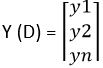
This cost function is used in the classification problems where there are multiple classes and input data belongs to only one class. Let us now understand how cross-entropy is calculated. Let us assume that the model gives the probability distribution as below for ‘n’ classes & for a particular input data D.
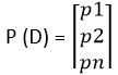
And the actual or target probability distribution of the data D is
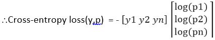
Then cross-entropy for that particular data D is calculated as
Cross-entropy loss(y,p) = – yT log(p)
= -(y1 log(p1) + y2 log(p2) + ……yn log(pn) )
Let us now define the cost function using the above example (Refer cross entropy image -Fig3),
p(Tomato) = [0.1, 0.3, 0.6]
y(Tomato) = [0, 0, 1]
Cross-Entropy(y,P) = – (0*Log(0.1) + 0*Log(0.3)+1*Log(0.6)) = 0.51
The above formula just measures the cross-entropy for a single observation or input data. The error in classification for the complete model is given by categorical cross-entropy which is nothing but the mean of cross-entropy for all N training data.
Categorical Cross-Entropy = (Sum of Cross-Entropy for N data)/N
2.2 Binary Cross Entropy Cost Function
Binary cross-entropy is a special case of categorical cross-entropy when there is only one output that just assumes a binary value of 0 or 1 to denote negative and positive class respectively. For example-classification between cat & dog.
Let us assume that actual output is denoted by a single variable y, then cross-entropy for a particular data D is can be simplified as follows –
Cross-entropy(D) = – y*log(p) when y = 1
Cross-entropy(D) = – (1-y)*log(1-p) when y = 0
The error in binary classification for the complete model is given by binary cross-entropy which is nothing but the mean of cross-entropy for all N training data.
Binary Cross-Entropy = (Sum of Cross-Entropy for N data)/N
Conclusion
Cost Function in Machine learning ,is a way to measure how well a model predicts outcomes. It’s crucial because it tells us how accurate our predictions are and guides us in improving the model’s performance. Different types of cost functions exist for tasks like predicting numbers or categories.
Frequently Asked Questions
The formula for the cost function in machine learning depends on the specific task and algorithm. For example, in linear regression, it might be the average of the squared differences between predicted and actual values.
The cost, as per the function, shows how much the model’s predictions differ from the actual outcomes. It tells us how accurate the model is.
The cost function, in short, is a way to measure how well a machine learning model is doing. It calculates the difference between what the model predicts and what actually happens, giving us an idea of its accuracy.
I hope you found this article helpful! Let me know what you think, especially if there are suggestions for improvement. You can connect with me on LinkedIn: https://www.linkedin.com/in/saily-shah/ and here’s my GitHub profile: https://github.com/sailyshah
The media shown in this article are not owned by Analytics Vidhya and is used at the Author’s discretion.


Shouldn't this " Error = y-y’ Where, Y – Actual Input Y’ – Predicted output " have Y - Actual output? Thank you for the article