Multicollinearity: Problem, Detection and Solution
Introduction
Multicollinearity, a common issue in regression analysis, occurs when predictor variables are highly correlated. This article navigates through the intricacies of multicollinearity, addressing its consequences, detection methods, and effective solutions. Understanding and managing multicollinearity is essential for accurate regression models and insightful data analysis. Explore the nuances of this challenge and enhance your statistical proficiency.
This article was published as a part of the Data Science Blogathon.
Table of contents
What is Multicollinearity?
One crucial assumption in regression models is that independent variables should not correlate among themselves. This is essential for isolating the individual impact of each variable on the target variable, as indicated by regression coefficients. Multicollinearity arises when variables are correlated, making it challenging to discern their separate effects on the target variable.
Why is Multicollinearity a Problem?
Multicollinearity causes the following 2 primary issues:
- Multicollinearity generates high variance of the estimated coefficients and hence, the coefficient estimates corresponding to those interrelated explanatory variables will not be accurate in giving us the actual picture. They can become very sensitive to small changes in the model.
- Consecutively the t-ratios for each of the individual slopes might get impacted leading to insignificant coefficients. It is also possible that the adjusted R squared for a model is pretty good and even the overall F-test statistic is also significant but some of the individual coefficients are statistically insignificant. This scenario can be a possible indication of the presence of multicollinearity as multicollinearity affects the coefficients and corresponding p-values, but it does not affect the goodness-of-fit statistics or the overall model significance.
How do we measure Multicollinearity?
A very simple test known as the VIF test is used to assess multicollinearity in our regression model. The variance inflation factor (VIF) identifies the strength of correlation among the predictors.
Now we may think about why we need to use ‘VIF’s and why we are simply not using the Pairwise Correlations.
Since multicollinearity is the correlation amongst the explanatory variables it seems quite logical to use the pairwise correlation between all predictors in the model to assess the degree of correlation. However, we may observe a scenario when we have five predictors and the pairwise correlations between each pair are not exceptionally high and it is still possible that three predictors together could explain a very high proportion of the variance in the fourth predictor.
Multicollinearity Formula
I know this sounds like a multiple regression model itself and this is exactly what VIFs do. Of course, the original model has a dependent variable (Y), but we don’t need to worry about it while calculating multicollinearity. The formula of VIF is:
VIF = 1 /(1- Rj2)
Here the Rj2 is the R squared of the model of one individual predictor against all the other predictors. The subscript j indicates the predictors and each predictor has one VIF. So more precisely, VIFs use a multiple regression model to calculate the degree of multicollinearity. Suppose we have four predictors – X1, X2, X3, and X4. So, to calculate VIF, all the independent variables will become dependent variables one by one. Each model will produce an R-squared value indicating the percentage of the variance in the individual predictor that the set of other predictors explain.
What is Variance inflation factor?
The term “variance inflation factor” (VIF) indicates the degree to which correlations among predictors inflate variance. For instance, a VIF of 10 means existing multicollinearity inflates coefficient variance tenfold compared to a model without multicollinearity. VIFs assess the precision of coefficient estimates, influencing the width of confidence intervals. Lower VIF values are preferable; values between 1 and 5 suggest manageable correlation, while those exceeding 5 indicate severe multicollinearity. Industry standards often recommend maintaining VIF below 5, although some texts consider VIF greater than 10 as severe, with judgment playing a role in deciding corrective measures.
How can we fix Multi-Collinearity in our model?
The potential solutions include the following:
- Simply drop some of the correlated predictors. From a practical point of view, there is no point in keeping 2 very similar predictors in our model. Hence, VIF is widely used as variable selection criteria as well when we have a lot of predictors to choose from.
- We can try to standardize the predictors by subtracting their mean from each of the observations. We can directly use these standardized variables in our model. The advantage of standardizing the variables is that the coefficients continue to represent the average change in the dependent variable given a 1 unit change in the predictor.
- Do some linear transformation e.g., add/subtract 2 predictors to create a new bespoke predictor.
- As an extension of the previous 2 points, another very popular technique is to perform Principal components analysis (PCA). PCA is used when we want to reduce the number of variables in our data but we are not sure which variable to drop. It is a type of transformation where it combines the existing predictors in a way only to keep the most informative part.
It then creates new variables known as Principal components that are uncorrelated. So, if we have 10-dimensional data then a PCA transformation will give us 10 principal components and will squeeze maximum possible information in the first component and then the maximum remaining information in the second component and so on. The primary limitation of this method is the interpretability of the results as the original predictors lose their identity and there is a chance of information loss. At the end of the day, it is a trade-off between accuracy and interpretability.
How to calculate VIF (R and Python Code)?
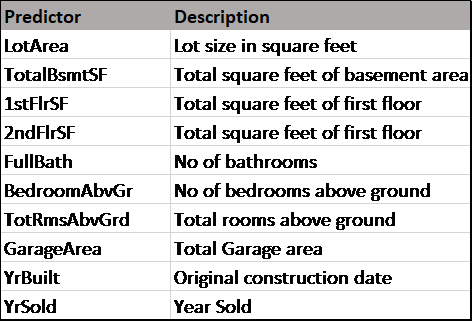
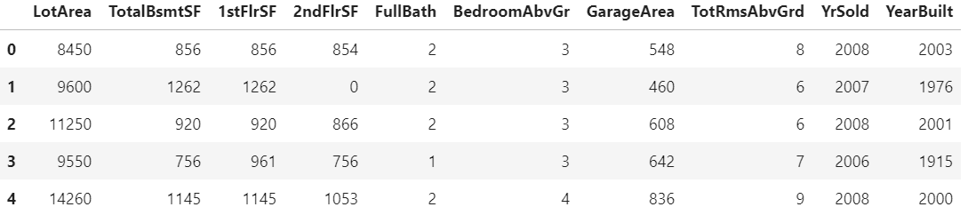
I am using a subset of the house price data from Kaggle. The dependent/target variable in this dataset is “SalePrice”. There are around 80 predictors (both quantitative and qualitative) in the actual dataset. For Simplicity’s purpose, I have selected 10 predictors based on my intuition that I feel will be suitable predictors for the Sale price of the houses. Please note that I did not do any treatment e.g., creating dummies for the qualitative variables. This example is just for representation purposes.
The following table describes the predictors I chose and their description.
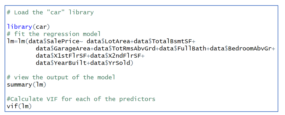
The below code shows how to calculate VIF in R. For this we need to install the ‘car’ package. There are other packages available in R as well.
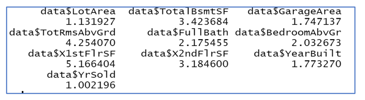
The output is shown below. As we can see most of the predictors have VIF <= 5
Now if we want to do the same thing in python then please see the code and output below
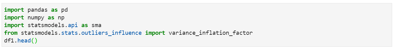
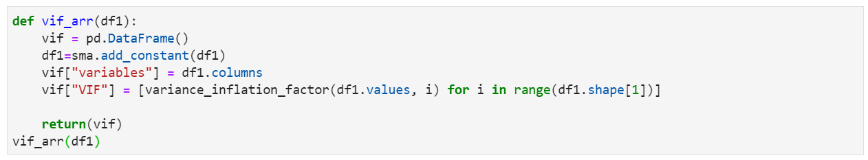
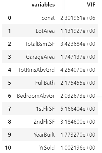
Please note that in the python code I have added a column of intercept/constant to my data set before calculating the VIFs. This is because the variance_inflation_factor function in python does not assume the intercept by default while calculating the VIFs. Hence, often we may come across very different results in R and Python output. For details, please see this discussion here.
Conclusion
In conclusion, understanding and addressing multicollinearity are crucial for robust regression models. Detecting signs, interpreting VIF values, and implementing corrective measures are essential. Mastering these skills is paramount for data scientists. Elevate your expertise further with our Blackbelt course, offering in-depth knowledge and practical applications in regression analysis. Enroll now for a seamless learning experience!
Frequently Asked Questions
A. Multicollinearity is the high correlation between independent variables in a regression model. It’s problematic because it undermines the model’s ability to distinguish individual effects of predictors.
A. Multicollinearity hampers the interpretability of regression coefficients by inflating standard errors, making it challenging to discern the unique impact of each variable on the dependent variable.
A. Multicollinearity is interpreted through variance inflation factor (VIF) values. High VIF values, typically above 5, indicate problematic multicollinearity, affecting the reliability of coefficient estimates.
A. Signs of multicollinearity include high pairwise correlations between predictors, coefficients changing signs when variables are added or removed, and inflated standard errors in regression results.


