Introducing Machine Learning for Spatial Data Analysis
This article discusses Machine Learning in Geographic Information System GIS, in other words, Machine Learning for spatial data analysis. Usually, we can find lots of Machine Learning applications and competitions for tabular, time series, text, and image data. We can also easily find tutorials or articles on Spatial Data Science, like in Analytics Vidhya, but they are mostly about visualizing spatial data or running basic spatial analysis, such as clip, buffer, and so on. There is a field specializing in integrating Machine Learning and GIS to solve many spatial problems. After reading this article, you will:
1. Understand the basic concept of Machine Learning and spatial analysis
2. Know Conventional Machine Learning and Machine Learning for spatial data analysis
If you are a Machine Learning user, this article aims to discuss and introduce (GIS) or spatial data analysis and how they can integrate. For GIS users, this article also introduces Machine Learning basics before exploring Machine Learning for spatial analysis.
Machine Learning
We will start by understanding the basics of Machine Learning. If you have understood the basic concept of Machine Learning, you may skip the following six paragraphs. As its name suggests, Machine Learning is used to build a model or a machine by asking it to learn from a big dataset. For today’s discussion, we will cover only tabular data and later spatial data, not including images and text. There are 3 types of Machine Learning. In this article, we will focus on only supervised and unsupervised learning.
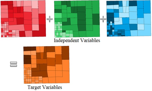
In supervised learning, we should have a training dataset and a test dataset. The training and test dataset are in tabular form with the columns as variables and the rows as observations. What makes them different is that the training dataset has one dependent/target variable, also usually named as a label, and the rest variables are independent variables. We train a model using a training dataset so that the model learns the pattern of independent variables to predict the target variable.
Test dataset, unlike training dataset, only contains independent variables without target variables. We use the Machine Learning model which has been trained with the training dataset to predict the missing target variable of the test dataset.
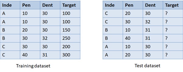
Training and test dataset
Supervised learning consists of regression and classification prediction. To predict the continuous target variable, we use regression. The categorical target variable is predicted using classification. There are many algorithms for regression and classification tasks. We will discuss them later.
Unsupervised learning is for a dataset that does not have a target variable. Unsupervised learning is not used to predict target variables, like supervised learning. Unsupervised learning is used to simplify large datasets according to the similarity of the observations and important variables. Please note that in this article, we use the term “variable” as a “feature”.
There are two types of unsupervised learning: clustering and dimensionality reduction. Clustering group observations into a number of clusters with a similar pattern. Dimensionality reduction computes how the variables can distinguish the observations. Variables that have mostly the same value are usually removed as they do not play an important role in the pattern. Since dimensionality reduction is not directly related to spatial analysis, we will not discuss it any longer in this article.
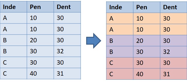
Clustering
Spatial Data Analysis
If you already have experience in Machine Learning, you may feel bored with the past six paragraphs. Now, we will study the basics of GIS. If you are a GIS user, you may skip the following 5 paragraphs. GIS includes collecting, managing, manipulating, analyzing, and visualizing spatial data as a system. In our material today, we will specifically focus on spatial analysis. Spatial data, unlike tabular data, has spatial attributes for each observation. There are two kinds of spatial data: vector and raster. Vector data can have point, line, or polygon shapes. raster data is composed of pixels as an image.
Spatial data is actually tabular data, but its observation has spatial attributes. In other words, each observation represents a location in the real world. As a result, observations in spatial data have latitudes, longitudes, areas (polygon), perimeters (polygon), centroids (polygon), and lengths (line). A group of spatial features can have density, distance, and centography (point). Tabular data does not have these.
Examples of polygon shape data are cities, residence blocks, land-use areas, and others. Road, pipeline, river, and route networks are expressed inline shapes. Point data usually contains information on elevation points, water table depth point, and other points of interest. Polygon, line, and point data can be converted to one another depending on what we need.
In tabular data, one observation does not have any spatial relationship with other observations. In spatial data, each observation has a distance from other observations. Due to the spatial attribute, we can operate spatial analysis (or geometric manipulation), such as clip, erase, buffer, union, interpolation, and many others.
“Clip” returns a group of observations of which the areas overlay on another group of observations. “Erase”, on the contrary, returns a group of observations of which the areas do not overlay another group of observations. “Buffer” creates a buffer area surrounding observations to a certain distance. “Union” unites more than one group of observations together. “Interpolation” creates interpolation between points to convert points into polygon shapes. Interpolation is related to Machine Learning since it predicts what the values are between the known points. We will discuss this more later.
Basic spatial data analysis
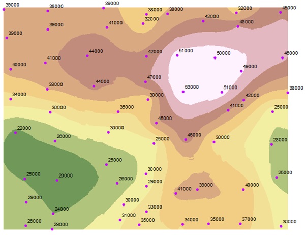
Basic Kriging interpolation
Machine Learning for Spatial Analysis
We can run Machine Learning tasks of regression, classification, and clustering in spatial data. As mentioned above, one of the frequently used GIS tools is interpolation, for instance interpolating a set of points containing house price information into polygon or raster. In fact, regression analysis in spatial data is for interpolation because we want to predict the unknown values in areas between the points.
The commonly used interpolation tool is Kriging. To interpolate the points using Machine Learning, we can try the tool Empirical Bayesian Kriging (EBK). Conventional Kriging only uses a single semivariogram model to predict unknown values, while EBK predicts unknown values using multiple semivariograms and the Bayesian rule.
The EBK explained above interpolates univariate data. We can also input dependent variables which influence the target variable. For example, inputting “distance from the main road”, “distance from the public facility”, “criminal occurrence”, and “disaster risk” can support house price interpolation using EBK. The other algorithms for spatial interpolation are Ordinary Least Squares (OLS) Regression and Geographically Weighted Regression (GWR).
Machine Learning for interpolation
Conventional Machine Learning Regression, like linear regression, tree-based regression, or Support Vector Machine regression, can also predict target variables according to the dependent variables, but cannot see that target variables in closer distance tend to have more similar values. The prices of houses in closer areas tend to be similar. Spatial interpolation follows the first law of geography invoked by Tobler: “near things are more related than distant things”.
Besides point interpolation, we can also perform Areal Interpolation. Areal interpolation returns a set of bigger polygons into a set of smaller polygons according to their surroundings. One polygon can be resampled into a few polygons with the values influenced by the neighboring values.
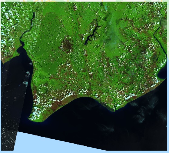
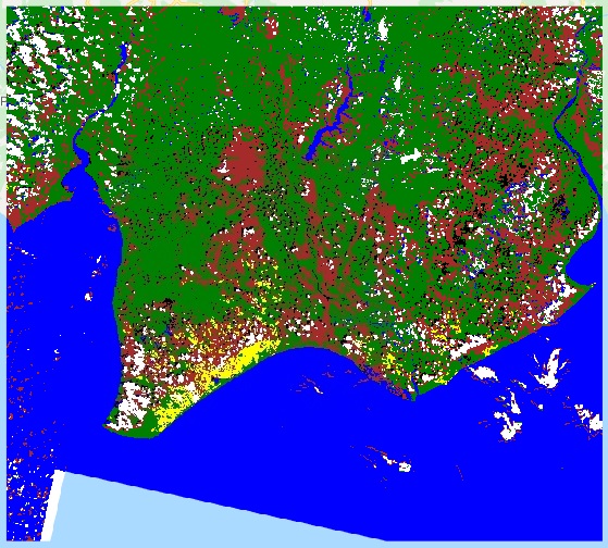
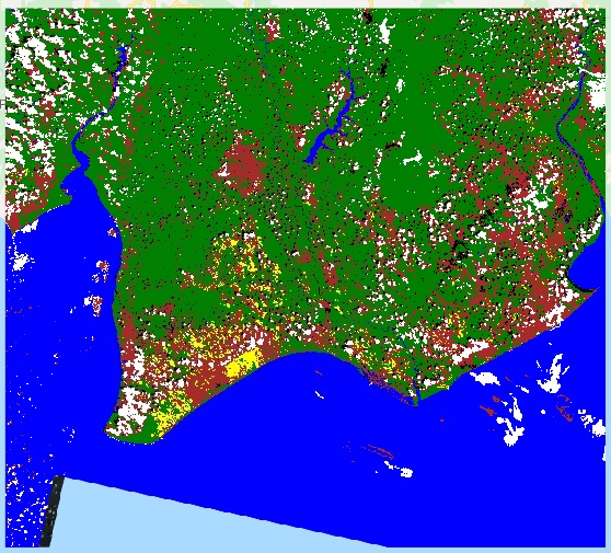
The second Machine Learning task is classification. In conventional Machine Leaning, we know Maximum Likelihood, Support Vector Machine, and Decision Tree for Classification. In the spatial analysis, the algorithm names are still the same. The popular task of Machine Learning for spatial classification is classifying land cover class from a satellite image. Remote Sensing is the branch of science studying this topic.
Another Machine Learning for spatial analysis we discuss today is clustering. In conventional Machine Learning, we can group a large number of observations into a few clusters according to the variables’ pattern similarity. We can also do the same thing for spatial data. But, as we have discussed before in regression technic, things located nearer to one another may be more similar. So, we can consider Spatially Constrained Multivariate Clustering. The “spatially constrained” ensures that each cluster groups a number of adjacent polygons. Polygons in the same cluster cannot be separated.
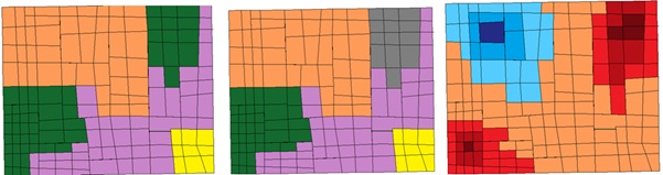
If we want to see where the high and low values are concentrated, we can apply Hot Spot Analysis. Hot Spot Analysis groups polygons into clusters to show where the high and low values are concentrated. The hot spot is where high values are concentrated and the cold spot is where low values are concentrated. See the illustration picture below of how the polygons are grouped into clusters using 3 different tools. Can you identify which one is which?
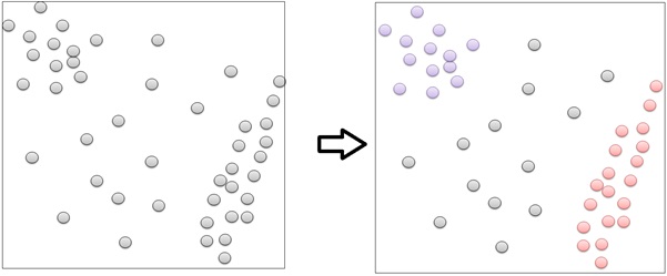
Density-based clustering is a Machine Learning tool specifically for point shape. This tool groups a number of points according to their density. A number of points gathering with high density are grouped into a cluster separating them from other points gathering far away. See the following points clustered according to their spatial density. This is the same as DBSCAN from conventional Machine Learning.
Not only vector data, but we can also cluster raster images using “Image Segmentation”. This tool segments objects in an image, usually satellite images or aerial photography. It is no different from conventional Machine Learning for image analysis. In conventional Machine Learning, we segment objects, such as people, trees, and houses in an image from any angle. In spatial data, we usually segment objects, like trees in a vertical image. The result then can be used for mapping.
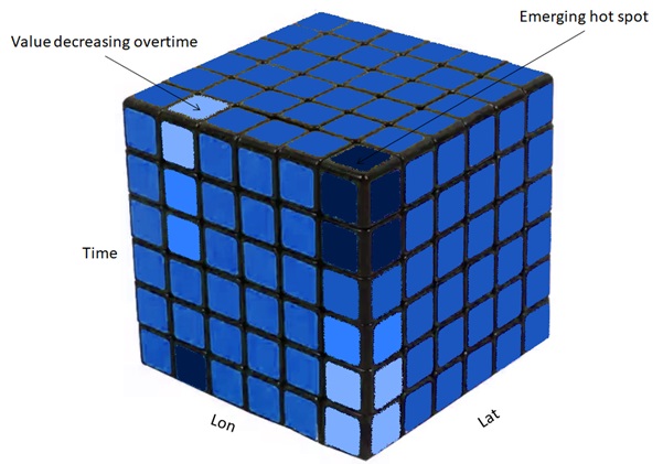
The last Machine Learning for spatial analysis for today’s discussion is Space-Time Pattern Mining. This tool clusters spatial and temporal data at the same time. The data is illustrated as 3-dimensional cuboid. The x and y-axis represent the spatial dimension and the z-axis is the time-series dimension. Each bin has a value. Then, we can analyze the emerging hot spots and cold spots. We can examine over time which area has increasing, decreasing, or constant value.
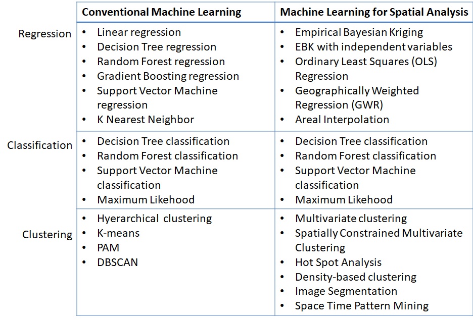
That is all about the intersection between Machine Learning and spatial analysis. Hopefully, we can gain insights from this article. Let’s broaden our knowledge from Machine Learning to spatial analysis or vice versa. The following shows conventional and Machine Learning for Spatial Analysis.
Summary
Machine Learning builds a predictive model from regression, classification, and clustering tasks. Spatial data, unlike tabular data, have all observations related spatially to one another. Machine Learning for spatial data analysis builds a model to predict, classify, or cluster unknown locations according to known locations in the training dataset by taking the spatial attribute into account.