Understanding Gradient Descent Algorithm

Objective

• Optimization is the core of every machine learning algorithm.
• Understand how the Gradient descent algorithm works and optimize model performance.

Note: If you are more interested in learning concepts in an Audio-Visual format, We have this entire article explained in the video below. If not, you may continue reading.

Introduction

Picture a scenario, you are playing a game with your friends where you have to throw a paper ball in a basket. What will be your approach to this problem?

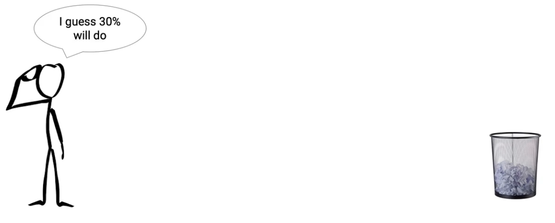
Here, I have a ball and basket at a particular distance, If I through the ball with 30% of my strength, I believe it should end up in the basket. But with this force ball didn’t reach the target and falls before the basket.

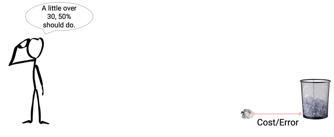
In my second attempt, I will use more power say 50% of my strength. This time I am sure it will reach its place. But unexpectedly ball crosses the basket and falls far from it.

Now I calculate and conclude the force should be somewhere and between 30% and 50%. This time I threw the ball with 45% of my strength and yay!  this time I succeed. The ball directly drops in the basket. That means 45% of strength is the optimum solution for this problem.

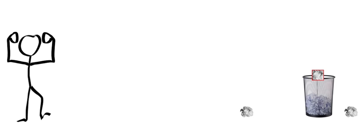
This is how the gradient descent algorithm works.

The intuition behind Gradient Descent Algorithm

Following up on the previous example let’s understand the intuition behind gradient descent.  As shown in the following image.

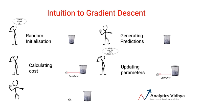
For a given problem statement, the solution starts with a Random initialization. These initial parameters are then used to generate the predictions i.e the output.  Once we have the predicted values we can calculate the error or the cost. i.e how far the predicted values are from the actual target. In the next step, we update the parameters accordingly and again made the predictions with updated parameters.

This process will go iteratively until we reach the optimum solution with minimal cost/error.

What is Gradient Descent?

Gradient descent is an optimization algorithm that works iteratively to find the model parameters with minimal cost or error values. If we go through a formal definition of Gradient descent

Gradient descent is a first-order iterative optimization algorithm for finding a local minimum of a differentiable function.

let’s consider a linear model, Y_pred= B0+B1(x). In this equation, Y_pred represents the output. B0 is the intercept and B1 is the slope whereas x is the input value.

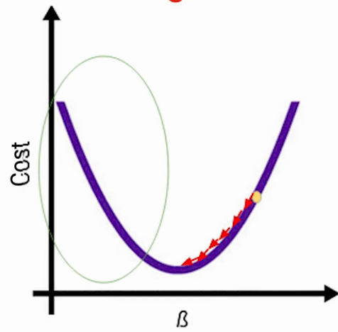
For a linear model, we have a convex cost function as shown in the image below that looks like a bowl.

Initially, you can start with randomly selected values of the parameters B0 and B1 and make the predictions Y_pred. The next step is to calculate the error i.e the difference between the original and the predictions.

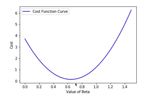
The predicted values with these parameters will land you anywhere on this cost function curve. Now the task is to update the value of B0 and B1 to minimize the error i.e coming down on this curve to the lower points. This process will continue until we reach the lowest point of this curve i.e the minimum cost.

Maths Behind Gradient descent

As by this time, we have a clear idea of Gradient descent, let’s now get into the mathematics behind it and see how it actually works in a step-wise manner.

Random Initialization and Generate Prediction

Here we are using a linear regression model. To start with a baseline model is always a great idea. In our baseline model, we are using the values 0 for B(slope of the line) and b (intercept) is the mean of all independent variables.

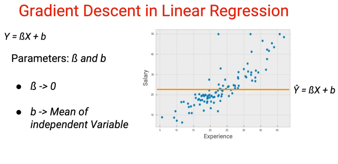
Now we can use this baseline model to have our predicted values y hat.

Calculate cost/error

Once we have our prediction we can use it in error calculation. Here, our error metric is the mean squared error(MSE).

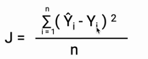
Mean squared error is the average squared difference between the estimated values and the actual value.

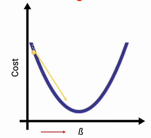
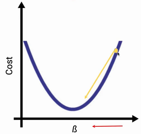
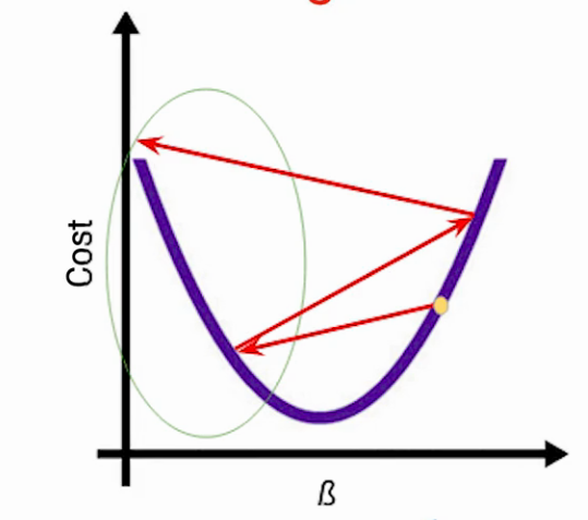
Our calculated error value of the baseline model can lead us anywhere on the Cost-B curve as shown in the following images. Now our task is to update B in such a way that it leads the error towards the bottom of the curve.

Update parameters

Now the question is how the parameters (B in this case) will be updated. To update our parameters we are going to use the partial derivatives. The partial derivatives give the slope of the line also, it is the change in the cost with respect to change in the B.

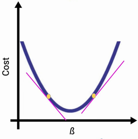
Look at the image below in each case the partial derivative will give the slope of the tangent. In the first case, the slope will be negative whereas in the other case the slope will be positive.

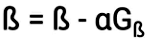
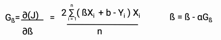
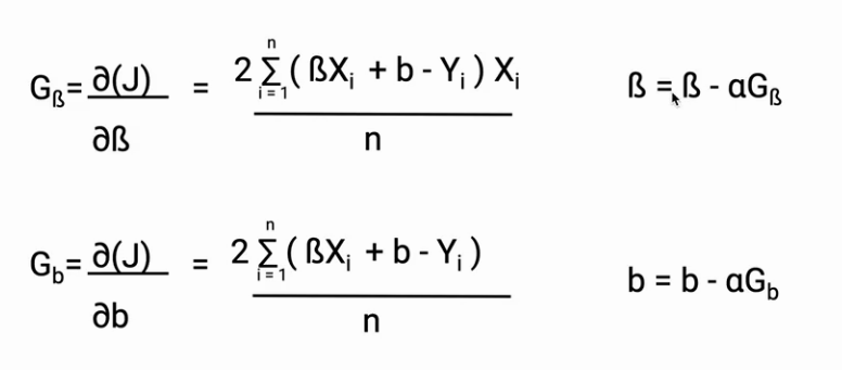
Once we have the partial derivative, we can update the values of B as shown in the image below.

Overall the whole process of updating the parameters will look like the following image.

Another important aspect of this whole process is the learning rate (a). The learning rate is a hyperparameter that decides the course and speed of the learning of our model.

The learning rate should be an optimum value. If the learning rate will be high, the steps taken will be large and we can miss the minima. As a result, the model will fail to converge.

On the other hand, if the learning rate will be too small, The model will take too much time to reach the minimum cost.

Effect of learning rate (a) too high learning rate (b) too low learning rate

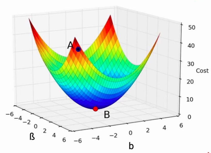
Now a question arises, what if there are multiple parameters in a model. In such cases, nothing will change just the dimensions of the cost function will increase. As it becomes a 3D plot in the following image. Also, the objective will remain the same i.e reaching the minima.

Further, the parameters will be updated exactly like the previous case as shown below.

Hence, it doesn’t matter how many parameters you have the process and objective will remain the same i.e to update the parameters to reach the minimum value of the cost function.

End Notes

In this article, we try to understand the gradient descent algorithm and the math behind it.

If you are looking to kick start your Data Science Journey and want every topic under one roof, your search stops here. Check out Analytics Vidhya’s Certified AI & ML BlackBelt Plus Program.

Connect with us in the comments below in case you have some queries.