Introduction
In a Neural Network, the Gradient Descent Algorithm is used during the backward propagation to update the parameters of the model. This article is completely focused on the variants of the Gradient Descent Algorithm in detail. Without any delay, let’s start!
Note: If you are more interested in learning concepts in an Audio-Visual format, We have this entire article explained in the video below. If not, you may continue reading.
Table of contents
Recap: What is the equation of the Gradient Descent Algorithm?
This is the updated equation for the Gradient Descent algorithm-
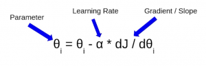
Here θ is the parameter we wish to update, dJ/dθ is the partial derivative which tells us the rate of change of error on the cost function with respect to the parameter θ and α here is the Learning Rate. I hope you are familiar with these terms, if not then I would recommend you to first go through this article on Understanding Gradient Descent Algorithm.
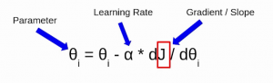
So, this J here represents the cost function and there are multiple ways to calculate this cost. Based on the way we are calculating this cost function there are different variants of Gradient Descent.
Batch Gradient Descent
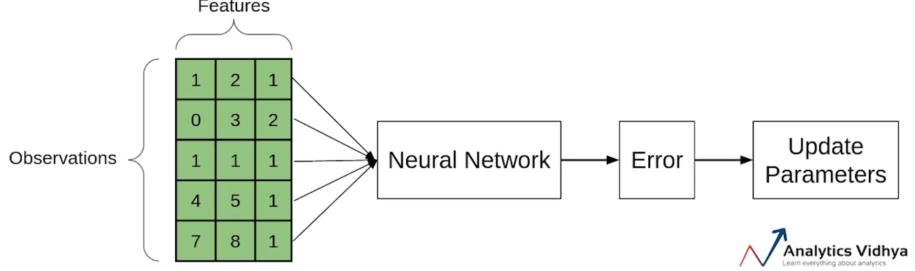
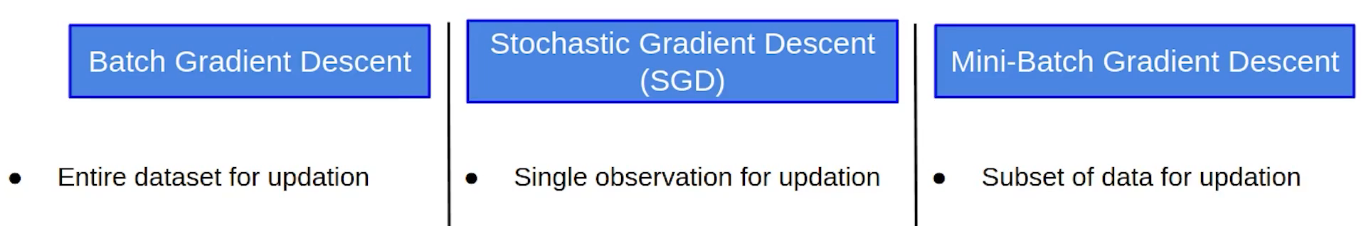
Let’s say there are a total of ‘m’ observations in a data set and we use all these observations to calculate the cost function J, then this is known as Batch Gradient Descent.
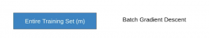
So we take the entire training set, perform forward propagation and calculate the cost function. And then we update the parameters using the rate of change of this cost function with respect to the parameters. An epoch is when the entire training set is passed through the model, forward propagation and backward propagation are performed and the parameters are updated. In batch Gradient Descent since we are using the entire training set, the parameters will be updated only once per epoch.
Stochastic Gradient Descent(SGD)
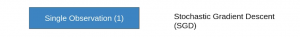
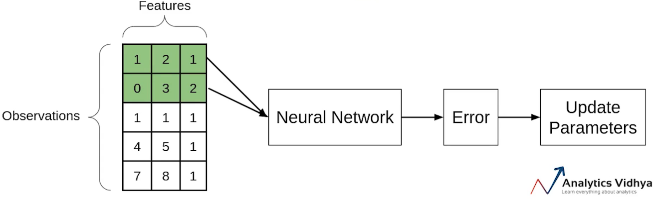
If you use a single observation to calculate the cost function it is known as Stochastic Gradient Descent, commonly abbreviated as SGD. We pass a single observation at a time, calculate the cost and update the parameters.
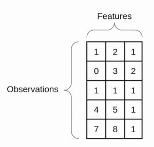
Let’s say we have 5 observations and each observation has three features and the values that I’ve taken are completely random.
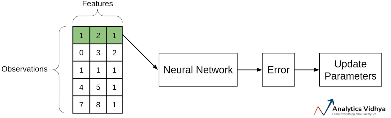
Now if we use the SGD, will take the first observation, then pass it through the neural network, calculate the error and then update the parameters.
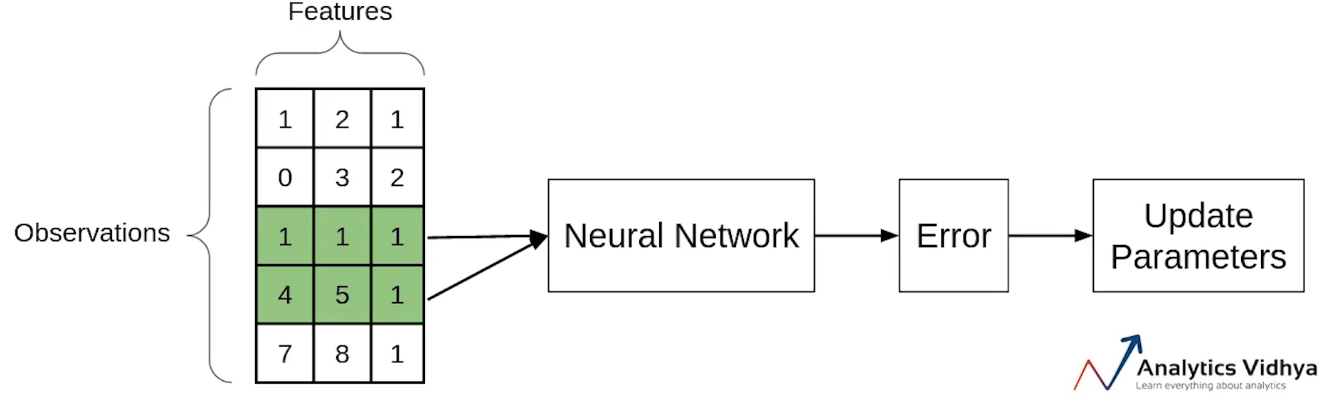
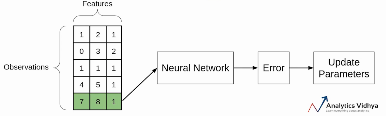
Then will take the second observation and perform similar steps with it. This step will be repeated until all observations have been passed through the network and the parameters have been updated.
Each time the parameter is updated, it is known as an Iteration. Here since we have 5 observations, the parameters will be updated 5 times or we can say that there will be 5 iterations. Had this been the Batch Gradient Descent we would have passed all the observations together and the parameters have been updated only once. In the case of SGD, there will be ‘m’ iterations per epoch, where ‘m’ is the number of observations in a dataset.
So far we’ve seen that if we use the entire dataset to calculate the cost function, it is known as Batch Gradient Descent and if use a single observation to calculate the cost it is known as SGD.
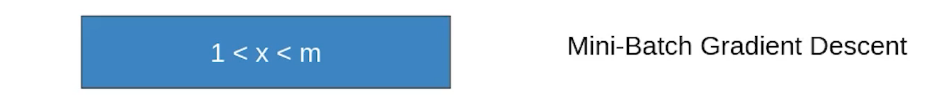
Mini-batch Gradient Descent
Another type of Gradient Descent is the Mini-batch Gradient Descent. It takes a subset of the entire dataset to calculate the cost function. So if there are ‘m’ observations then the number of observations in each subset or mini-batches will be more than 1 and less than ‘m’.
Again let’s take the same example. Assume that the batch size is 2. So we’ll take the first two observations, pass them through the neural network, calculate the error and then update the parameters.
Then we will take the next two observations and perform similar steps i.e will pass through the network, calculate the error and update the parameters.
Now since we’re left with the single observation in the final iteration, there will be only a single observation and will update the parameters using this observation.
Comparison between Batch GD, SGD, and Mini-batch GD:
This is a brief overview of the different variants of Gradient Descent. Now let’s compare these different types with each other:
Comparison: Number of observations used for Updation
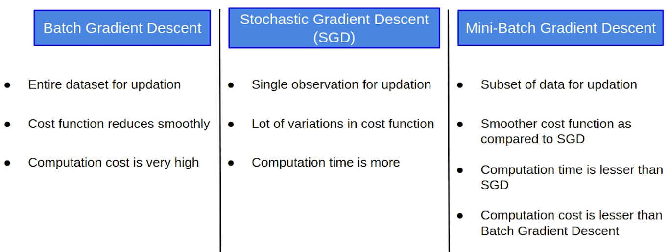
- In batch gradient Descent, as we have seen earlier as well, we take the entire dataset > calculate the cost function > update parameter.
- In the case of Stochastic Gradient Descent, we update the parameters after every single observation and we know that every time the weights are updated it is known as an iteration.
- In the case of Mini-batch Gradient Descent, we take a subset of data and update the parameters based on every subset.
Comparison: Cost function
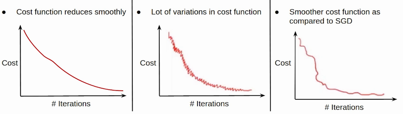
- Now since we update the parameters using the entire data set in the case of the Batch GD, the cost function, in this case, reduces smoothly.
- On the other hand, this updation in the case of SGD is not that smooth. Since we’re updating the parameters based on a single observation, there are a lot of iterations. It might also be possible that the model starts learning noise as well.
- The updation of the cost function in the case of Mini-batch Gradient Descent is smoother as compared to that of the cost function in SGD. Since we’re not updating the parameters after every single observation but after every subset of the data.
Comparison: Computation Cost and Time
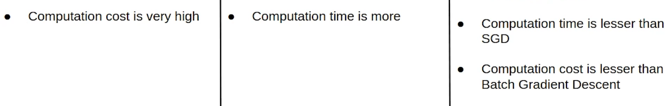
- Now coming to the computation cost and time taken by these variants of Gradient Descent. Since we’ve to load the entire data set at a time, perform the forward propagation on that and calculate the error and then update the parameters, the computation cost in the case of Batch gradient descent is very high.
- Computation cost in the case of SGD is less as compared to the Batch Gradient Descent since we’ve to load every single observation at a time but the Computation time here increases as there will be more number of updates which will result in more number of iterations.
- In the case of Mini-batch Gradient Descent, taking a subset of the data there are a lesser number of iterations or updations and hence the computation time in the case of mini-batch gradient descent is less than SGD. Also, since we’re not loading the entire dataset at a time whereas loading a subset of the data, the computation cost is also less as compared to the Batch gradient descent. This is the reason why people usually prefer using Mini-batch gradient descent. Practically whenever we say Stochastic Gradient Descent we generally refer to Mini-batch Gradient Descent.
Here is the complete Comparison Chart:
FAQs
Q1.Which is the fastest gradient descent?
The fastest gradient descent algorithm is stochastic gradient descent (SGD), as it updates the model parameters after processing each training example, leading to faster convergence.
Q2. Why is batch gradient descent better?
Batch gradient descent is better because it computes the gradient using the entire training dataset, leading to more accurate updates and smoother convergence. However, it can be slower than stochastic gradient descent, especially for large datasets
Q3. How is batch gradient descent different from normal equation?
Batch gradient descent is an iterative algorithm that updates the model parameters after processing the entire training dataset, while the normal equation is a closed-form solution that directly computes the optimal parameters without iteration.
End Notes
In this video, we saw the variants of the Gradient Descent Algorithm in detail. We also compared all of them with each other and found that Mini-batch GD is the most commonly used variant of the Gradient Descent.
If you are looking to kick start your Data Science Journey and want every topic under one roof, your search stops here. Check out Analytics Vidhya’s Certified AI & ML BlackBelt Plus Program
Let us know if you have any queries in the comments below regarding edge detection.
Himanshi Singh
07 Nov, 2023
I am a data lover and I love to extract and understand the hidden patterns in the data. I want to learn and grow in the field of Machine Learning and Data Science.


Very informative. Thanks
Hi HS13, It is really nice article with less content, you have explained very well. Please keep this rolling on. Few request: 1. Can you put more videos similar like this? 2. Can you also share the source code for each variation of GD algo? Thank you
very comprehensive tutorial....excellent and keep it up
Really nice article!!