What is Feature Extraction and Feature Extraction Techniques

Table of contents
What is Feature Extraction?
Feature extraction is the process of identifying and selecting the most important information or characteristics from a data set. It’s like distilling the essential elements, helping to simplify and highlight the key aspects while filtering out less significant details. It’s a way of focusing on what truly matters in the data.
Why feature Extraction is essential?
Feature extraction is important because it makes complicated information simpler. In things like computer learning, it helps find the most crucial patterns or details, making computers better at predicting or deciding things by focusing on what matters in the data.
Common Feature Extraction Techniques
1. The need for Dimensionality Reduction
In real-world machine learning problems, there are often too many factors (features) on the basis of which the final prediction is done. The higher the number of features, the harder it gets to visualize the training set and then work on it. Sometimes, many of these features are correlated or redundant. This is where dimensionality reduction algorithms come into play.
2. What is Dimensionality reduction
Dimensionality reduction is the process of reducing the number of random features under consideration, by obtaining a set of principal or important features.
Dimensionality reduction can be done in 2 ways:
a. Feature Selection: By only keeping the most relevant variables from the original dataset
i. Correlation
ii. Forward Selection
iii. Backward Elimination
iv. Select K Best
v. Missing value Ratio
Please refer to this link for more information on the Feature Selection technique
b. Feature Extraction: By finding a smaller set of new variables, each being a combination of the input variables, containing basically the same information as the input variables.
i. PCA(Principal Component Analysis)
ii. LDA(Linear Discriminant Analysis)

In this article, we will mainly focus on the Feature Extraction technique with its implementation in Python.
The feature Extraction technique gives us new features which are a linear combination of the existing features. The new set of features will have different values as compared to the original feature values. The main aim is that fewer features will be required to capture the same information. We might think that choosing fewer features might lead to underfitting but in the case of the Feature Extraction technique, the extra data is generally noise.
The feature extraction in machine learning technique provides us with new features, forming a linear combination of the existing ones. This results in a new set of features with values different from the original ones. The primary objective is to require fewer features to capture the same information. While one might assume that opting for fewer features could lead to underfitting, in the case of the feature extraction technique, the additional data is typically considered noise.
3. PCA(Principal Component Analysis)
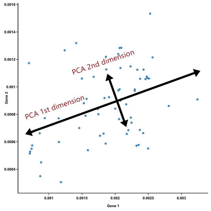
In simple words, PCA is a method of obtaining important variables (in form of components) from a large set of variables available in a data set. It tends to find the direction of maximum variation (spread) in data. PCA is more useful when dealing with 3 or higher-dimensional data.
PCA can be used for anomaly detection and outlier detection because they will not be part of the data as it would be considered noise by PCA.Building PCA from scratch:
- Standardize the data (X_std)
- Calculate the Covariance-matrix
- Calculate the Eigenvector & Eigenvalues for the Covariance-matrix.
- Arrange all Eigenvalues in decreasing order.
- Normalize the sorted Eigenvalues.
- Horizontally stack the Normalized_ Eigenvalues =W_matrix
- X_PCA=X_std .dot (W_matrix)
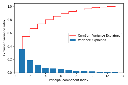
We can infer from the above figure that from the first 6 Principal Components we are able to capture 80% of the data. This shows us the Power of PCA that with only using 6 features we able to capture most of the data.
A principal component is a normalized linear combination of the original features in a data set.
The first principal component(PC1) will always be in the direction of maximum variation and then the other PC’s follow.
We need to note that all the PC’s will be perpendicular to each other. The main intention behind this is that no information present in PC1 will be present in PC2 when they are perpendicular to each other.
Implementation of PCA using Python
For this, I have used the Wine dataset. In this part, I have implemented the PCA along with Logistic regression followed by Hyperparameter Tuning.
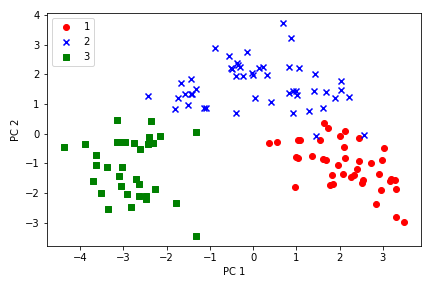
a. First we standardize the data and apply PCA. Then I have plotted the result to check the separability.
b. Then I have applied Logistics Regression and plotted with the help of the Decision boundary for the train and test data.
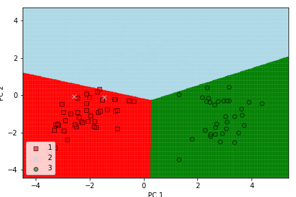
Decision Boundary for Train data
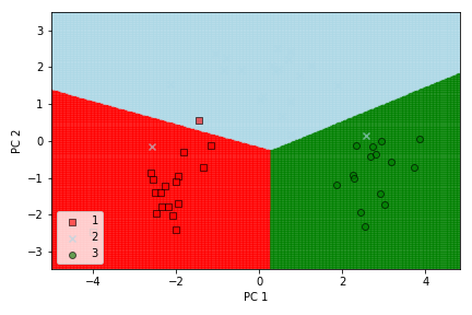
Decision Boundary for Test data
c. Finally I had applied Hyperparameter Tuning with Pipeline to find the PC’s which have the best test score.
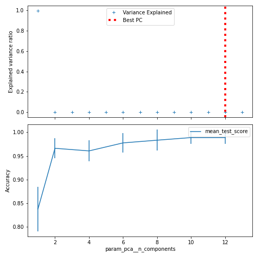
Hyperparameter Tuning
4. Kernel PCA
We know that PCA performs linear operations to create new features. PCA fails when the data is non-linear and is not able to create the hyperplane.
This is where Kernel PCA comes to our rescue. It is similar to SVM in the way that it implements Kernel–Trick to convert the non-linear data into a higher dimension where it is separable.
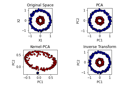
Kernel PCA
In the above figure we can see that PCA is not able to separate non-linear data but with the help of Kernel -PCA it is able to generate class-separability.
5. Disadvantages of PCA:
PCA does not guarantee class separability which is why it should be avoided as much as possible which is why it is an unsupervised algorithm. In other words, PCA does not know whether the problem which we are solving is a regression or classification task. That is why we have to be very careful while using PCA.
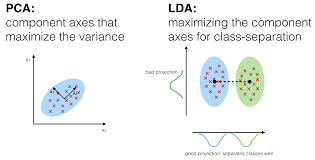
LDA v/s PCA
6. LDA
Though PCA is a very useful technique to extract only the important features but should be avoided for supervised algorithms as it completely hampers the data.
If we still wish to go for Feature Extraction Technique then we should go for LDA instead.
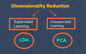
The main difference between LDA and PCA is:
1. LDA is supervised PCA is unsupervised.
2. LDA =Describes the direction of maximum separability in data.PCA=Describes the direction of maximum variance in data.
3. LDA requires class label information unlike PCA to perform fit ().
LDA works in a similar manner as PCA but the only difference is that LDA requires class label information, unlike PCA.
Implementation of LDA using Python
a. I have first standardized the data and applied LDA.
b. Then I have used a linear model like Logistic Regression to fit the data. Then plotted the Decision Boundary for better class separability understanding
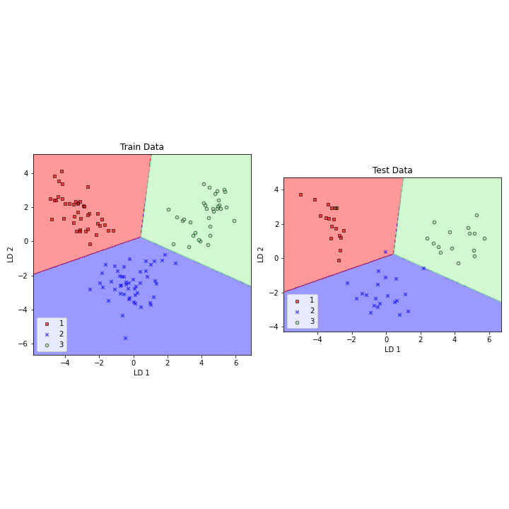
LDA with Logistic Regression
Note: We can see that LDA is a linear model and passing the output of one linear model to another does no good. It is better to try passing the output of the linear model to a nonlinear model.
From the above figure, we were able to achieve an accuracy of 100% for the train data and 98% for the test data.
c. Thus, this time we have used a nonlinear model (SVM) to prove the above.
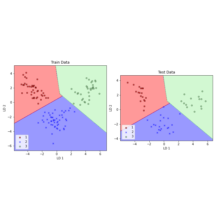
LDA with SVM
From the above figure, we were able to achieve an accuracy of 100% for both the test and train data.
Thus we can see that passing linear input to a nonlinear model is more beneficial instead.
Conclusion
Feature Extraction, essential for data analysis, involves techniques like Principal Component Analysis (PCA) for Dimensionality Reduction. By reducing complexity, it enhances efficiency, making it a crucial tool in extracting meaningful patterns from data for better insights and decision-making.
For the Code, implementation refer to my GitHub link: Dimensionality Reduction Code Implementation in Python
Hope you find this article informative. I’m looking forward to hearing your views and ideas in the comments section.
Frequently Asked Questions
The best algorithm depends on the task. Popular ones are PCA, t-SNE, and Autoencoders. Choose based on specific needs.
In Machine Learning (ML), people manually pick and create features, following set rules. It involves choosing a limited number of features based on human expertise.
In Deep Learning (DL), the computer figures out which features are important by itself. DL handles a large number of raw features, and the model learns to extract and represent features, reducing the need for human-defined rules


