This article was published as a part of the Data Science Blogathon.
Introduction
Hello readers!
In our routine life, we come across a lot of statistics that vary to and fro. The prominent ones being the environmental factors such as temperature, humidity level, the amount of rainfall, etc. These factors generally change many a time during the day.
Apart from these, we visit many shops which sell various types of items and keep a record of their sales either daily or monthly
Now, what is the common feature in all such types of data and how can this data be pre-processed before applying any suitable model to it?
In this article, we will get the answer to such questions and see what criteria such dataset follow and how these criteria can be monitored in the python language.
Table of Contents
- Objective
- Overview
- Data Stationarity
- Method to check Stationarity of data
- Implementation of code
- Observation
- Conclusion
Objective –To examine the stationarity of time series data in python by comparing two different datasets with the help of two test Rolling statistics and Augmented Dickey – fuller test.
Overview-
Time Series data -The set of observations that are collected at the regular intervals of time form a time series data. It tells the magnitude of data collected over a period of time. For example, you have data of a mobile store that describes the total sale of mobile phones per day or data of the amount of rainfall per day of a particular place, such types of data are called time series data where one of the variables is the time.
The time-series data must be in equal intervals of time as a day, a month, a week, a decade, etc.
Uses:-
- Time series data is used to predict future data values with the help of previous data.
- It helps to forecast the business opportunity in the future by analyzing the previous sales data, observing the previous trend, analyzing the past behavior, etc.
- It helps to evaluate the current accomplishment.
Patterns in time series
They are 3 types of patterns that are usually observed in time series data:-
1) Trend: – It describes the movement of data values either higher or lower at regular intervals of time over a long period. If the movement of data value is in the upper pattern, then it is known as an upward trend and if the movement of data value shows a lower pattern then it is known as a downward trend. If the data values show a constant movement, then is known as a horizontal trend.
2) Seasonality: – It is a continuous upward and downward trend that repeat itself after a fixed interval of time.
3) Irregularity: – It has no systematic pattern and occurs only for a short period of time and it does not repeat itself after a fixed interval of time. It can also be known as noise or residual.
Stationarity
The Time series data model works on stationary data. The stationarity of data is described by the following three criteria:-
1) It should have a constant mean
2) It should have a constant variance
3) Auto covariance does not depend on the time
*Mean – it is the average value of all the data
*Variance – it is a difference of each point value from the mean
*Auto covariance –it is a relationship between any two values at a certain amount of time.
Method to check the stationarity of the Time Series Data:-
There are two methods in python to check data stationarity:-
1) Rolling statistics:-
This method gave a visual representation of the data to define its stationarity. A Moving variance or moving average graph is plot and then it is observed whether it varies with time or not. In this method, a moving window of time is taken (based on our needs, for eg-10, 12, etc.) and then the mean of that time period is calculated as the current value.
2) Augmented Dickey- fuller Test (ADCF): –
In this method, we take a null hypothesis that the data is non-stationary. After executing this test, it will give some results comprised of test statistics and some other critical values that help to define the stationarity. If the test statistic is less than the critical value then we can reject the null hypothesis and say that the series is stationary.
Implementation of Code Data set Description
Dataset 1:- Monthly electricity production
Dataset 2:- Monthly sunspots
#Importing modules
import numpy as np
import pandas as pd
import matplotlib.pylab as plt
%matplotlib inline
#Loading Datasets


data=pd.read_csv(r'C:UsersnishthaDesktopelec.csv')

data1=pd.read_csv(r'C:UsersnishthaDesktopmonthly-sunspots.csv')
Converting data into date time format
#Dataset1:-
data['DATE']=pd.to_datetime(data['DATE'],infer_datetime_format=True)
index=data.set_index(['DATE'])
from datetime import datetime
index.head()
#Dataset2:-
data1['Month']=pd.to_datetime(data1['Month'],infer_datetime_format=True)
index1=data1.set_index(['Month'])
from datetime import datetime
index1.head()
Plotting the graphs
#Dataset 1:-
plt.xlabel("DATE")
plt.ylabel("Electric Production")
plt.plot(index)
Dataset 2:-
Python Code:
.png)
#Augmented Dickey-fuller test
#Dataset1
from statsmodels.tsa.stattools import adfuller
print("Observations of Dickey-fuller test")
dftest = adfuller(data['prod'],autolag='AIC')
dfoutput=pd.Series(dftest[0:4],index=['Test Statistic','p-value','#lags used','number of observations used'])
for key,value in dftest[4].items():
    dfoutput['critical value (%s)'%key]= value
print(dfoutput)
Observations of Dickey-fuller test
Test Statistic                  -2.256990
p-value                          0.186215
#lags used                      15.000000
number of observations used    381.000000
critical value (1%)             -3.447631
critical value (5%)             -2.869156
critical value (10%)            -2.570827
dtype: float64
#Dataset2
from statsmodels.tsa.stattools import adfuller
print("Observations of Dickey-fuller test")
dftest = adfuller(data1['Sunspots'],autolag='AIC')
dfoutput=pd.Series(dftest[0:4],index=['Test Statistic','p-value','#lags used','number of observations used'])
for key,value in dftest[4].items():
    dfoutput['critical value (%s)'%key]= value
print(dfoutput)
Observations of Dickey-fuller test
Test Statistic                -9.567668e+00
p-value                        2.333452e-16
#lags used                     2.700000e+01
number of observations used    2.792000e+03
critical value (1%)           -3.432694e+00
critical value (5%)           -2.862576e+00
critical value (10%)          -2.567321e+00
dtype: float64
#Rolling Statistics Test
#Dataset1
rmean=index.rolling(window=12).mean()
rstd=index.rolling(window=12).std()
print(rmean,rstd)
orig=plt.plot(index , color='black',label='Original')
mean= plt.plot(rmean , color='red',label='Rolling Mean')
std=plt.plot(rstd,color='blue',label = 'Rolling Standard Deviation')
plt.legend(loc='best')
plt.title("Rolling mean and standard deviation")
plt.show(block=False)
.png)
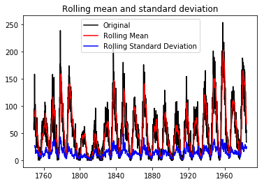
#dataset2
rmean1=index1.rolling(window=12).mean()
rstd1=index1.rolling(window=12).std()
print(rmean1,rstd1)
orig=plt.plot(index1 , color='black',label='Original')
mean= plt.plot(rmean1 , color='red',label='Rolling Mean')
std=plt.plot(rstd1,color='blue',label = 'Rolling Standard Deviation')
plt.legend(loc='best')
plt.title("Rolling mean and standard deviation")
plt.show(block=False)
Observation
We observed the following things on two datasets after implementing both the test.
Augmented dickey-fuller test :
The result of the dickey-fuller test consists of some values like test statistics, p-value critical values, etc. For dataset1 the test statistic value (-2.25) is not less than the critical values (-3.44 , -2.86 , -2.57) at different percentage . In this case, we cannot reject our null hypothesis and conclude that our data is not stationary,
For dataset2, the test statistics value (-9.56) is less than the critical values (-3.43,-2.87,-2.56) at different percentage. In this case, we can reject our null hypothesis conclude that our data is stationary.
Rolling Statistics Test :
The Rolling statistics test gives the visual representation of the dataset.
For the first dataset, the graph of rolling mean and rolling standard deviation is not constant, this shows that our first dataset is not stationary while for the second dataset graph of rolling mean and rolling standard deviation is constant, this shows that our second dataset is stationary.
Conclusions
Both tests can be used to check the stationarity of the data. The Rolling statistic test gives the pictorial representation while the dickey-fuller test gives some values which help to determine whether data is stationary or not.
The media shown in this article are not owned by Analytics Vidhya and is used at the Author’s discretion.
Nishtha Arora
26 Aug, 2022


