The most common way to load a CSV file in Python is to use the DataFrame of Pandas.
import pandas as pd
testset = pd.read_csv(testset_file)
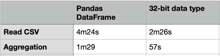
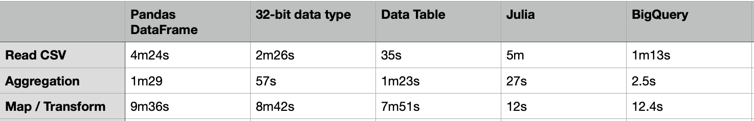
The above code took about 4m24s to load a CSV file of 20G.
Data analysis can be easily done with the DataFrame. e.g. for data aggregation, it can be done by the code below:
testset[["passband","flux"]].groupby(by=["passband"]).mean()
It took about 1m29s to compute the aggregated table group by “passband”.
One way to load the CSV file faster is to use the 32-bit data type. The code below just took 2m26s to load the same 20G CSV file, which is almost 2X faster. For the same group-by aggregation, it just took 57s, which is also much faster.
%%time
thead = pd.read_csv(testset_file, nrows=5) # just read in a few lines to get the column headers
dtypes = dict(zip(thead.columns.values, ['int32', 'float32', 'int8', 'float32', 'float32', 'bool']))   # datatypes as given by the data page
del thead
print('Datatype used for each column:n', json.dumps(dtypes))
testset = pd.read_csv(testset_file, dtype=dtypes)
testset.info()
To transform the data in the DataFrame, we can apply the transform function on each row. e.g. To compute a new column “ff” by multiplying 2 columns: “flux” and “flux_err”, it can be done by the following code:
%%time
testset["ff"] = testset[["flux","flux_err"]].apply(lambda x: x[0]*x[1], axis=1)
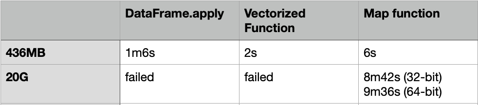
However, it only works if your dataset is not very large. In our case of 20G, the operation cannot be finished and the Jupyter notebook kernel was self-restarted. My testing machine is the iMac with just 8G memory. It likely had insufficient memory. I also tried the same transform on the DataFrame of 32-bit data types, it resulted in self-restart as well.
DataFrame.apply is slow, even for a 436MB CSV file, it still took 1m6s to finish. To make it faster, we can convert the DataFrame into NumPy array, and then use the Vectorized function or the function: “map” to apply the transform.
Here is the code of the Vectorized function:
f = lambda x,y: x*y
vf = np.vectorize(f)
%%time vf(testset["flux"].values,testset["flux_err"].values)
Here is the code of the “Map” function:
%%time
testset["ff"] = list(map(lambda x:x[0]*x[1], testset[["flux","flux_err"]].values ) )
The Vectorized function took about 2s to complete, while the “Map” function took about 6s to complete.
How about we use the same NumPy method for the 20G CSV file?
For the Vectorized function, it also failed with self-restart for using both the 32-bit and 64-bit data types.
The “Map” function can be finished with 8m42s and 9m36s for using the 32-bit and 64-bit data types respectively. That means the “Map” function on the NumPy array is using much less memory.
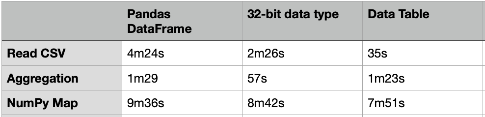
Apart from the Pandas DataFrame, there are many other packages that we can load and process with a large volume of data. One of them is the “Data Table” which is much faster than DataFrame. The usage of the Data Table is similar to the DataFrame, but it just needs 35s to load the same 20G CSV file.
import datatable as dt
from datatable import (dt, f, by, ifelse, update, sort,
                       count, min, max, mean, sum, rowsum)
%%time dt_df = dt.fread(testset_file)
%%time dt_df[:, mean(f.flux), by('passband')]
Nevertheless, the above group-by aggregation just took 1m23s, which is similar to the performance of the DataFrame.
Although the Data Table does not have any transform function similar to the DataFrame.apply, we can still use the same NumPy conversion with the “Map” function to apply the transform.
%%time
dt_df[:,"ff_num"] = np.array(list(map(lambda x:x[0]*x[1], dt_df[:,["flux","flux_err"]].to_numpy() ) ))
It took about 7m51s to complete, which is 18% faster than the same case in the DataFrame.
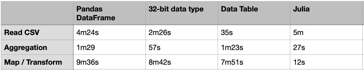
Apart from Python, another programming language emerging in the area of Data Science is “Julia”. “Julia” is a high performant language. Here is the code for loading the same CSV file, doing the same group-by aggregation, and the same transform function.
using DataFrames
using CSV
@time df = DataFrame(CSV.File(file; types=Dict(:object_id => Int32, :mjd => Float32, :passband => Int8,:flux => Float32, :flux_err => Float32, :detected => Bool)))
@time df_mean = combine(groupby(df,:passband),:flux => mean => :mean)
@time transform!(df, [:flux,:flux_err] => ByRow(*) => :Err)
The result is:
Although it took a similar time to load the CSV file, the aggregation and the transform are really fast. Most importantly, the memory footprint is much smaller when compared to Python, which cannot even finish the transform function due to insufficient memory. We need to convert the DataFrame to NumPy array to use the “Map” function for Data transformation, but it still took much slower than Julia. Julia transform is 48X faster!
Another good choice for big data analytics is to leverage cloud solutions such as GCP Big Query.
First of all, we need to upload the CSV file to Cloud Storage. It can be done efficiently with multi-thread in parallel and with compression.
gsutil -o "GSUtil:max_upload_compression_buffer_size=8G" -m cp -J test_set.csv gs://<bucket-name>
Once the data has been copied to the Cloud Storage, it can be easily uploaded to the BigQuery table, and perform the aggregation and transform function using SQL.
SELECT passband,avg(flux) FROM `iwasnothing-self-learning.myloadtest.df` group by passband;
SELECT object_id, flux*flux_err as ff FROM `iwasnothing-self-learning.myloadtest.df` ;
The SQL output can be set to the destination table to store the final result.
Result:
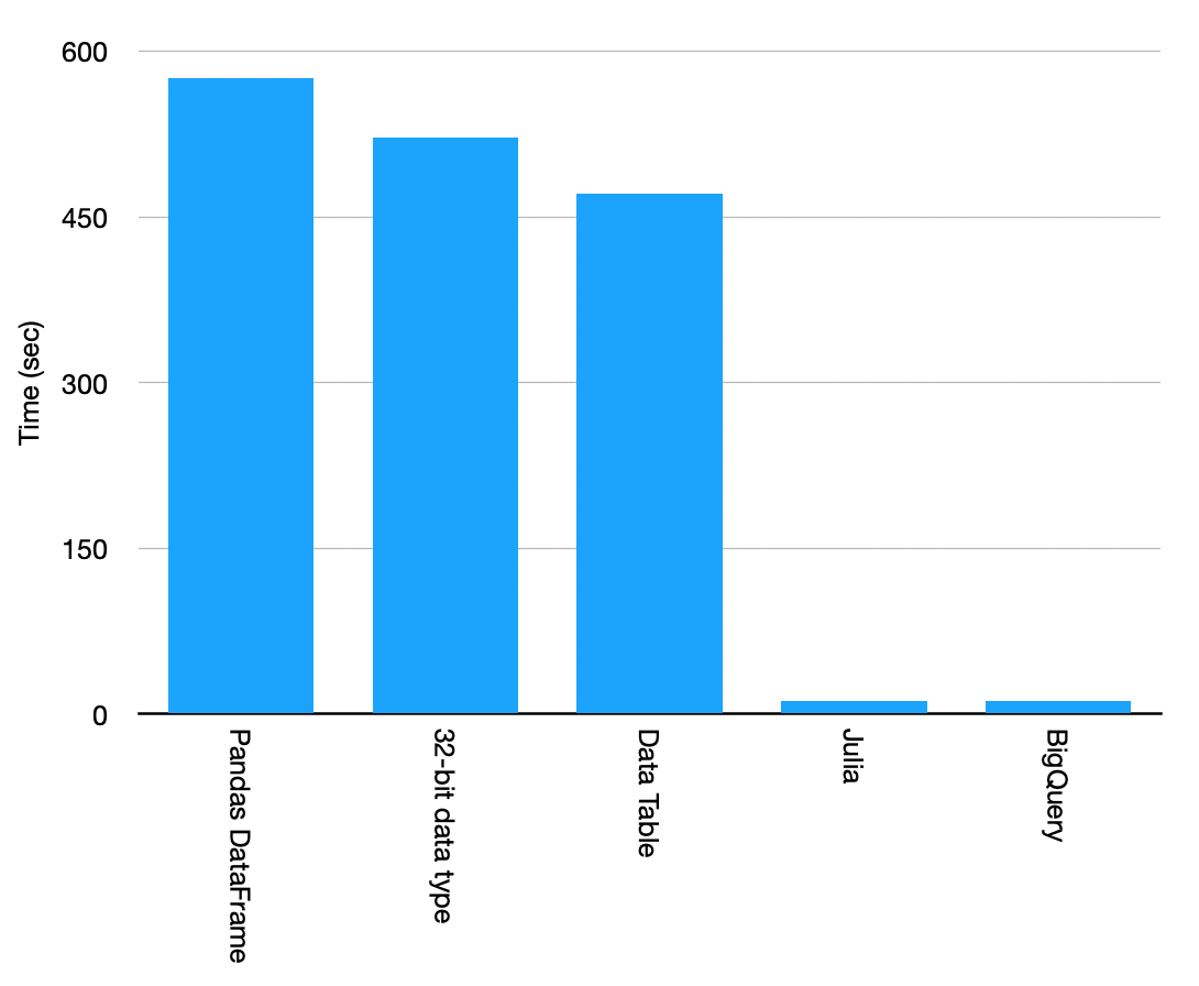
As the final result, the Cloud Solution wins.
Lorem ipsum dolor sit amet, consectetur adipiscing elit,


Thank you for posting. I am involved in development of DataFrames.jl in Julia. Therefore I would like to ask two questions: could you re-run the benchmark using DataFrames.jl 1.0 release (you seem to be using DataFrames.jl 0.22). Also with how many threads have you started your Julia session? (as clearly BigQuery performs distributed computations). Thank you! (alternatively I can re-run your benchmarks on latest DataFrames.jl if you would be so kind to share the source data)