K-Mean: Getting the Optimal Number of Clusters
Introduction
In this beginner’s tutorial on data science, we will discuss about determining the optimal number of clusters in a data set, which is a fundamental issue in partitioning clustering, such as k-means clustering. K-means clustering is an unsupervised learning machine learning algorithm. In an unsupervised algorithm, we are not interested in making predictions (since we don’t have a target/output variable). The objective is to discover interesting patterns in the data, e.g., are there any subgroups or ‘clusters’ among the bank’s customers?
Clustering techniques use raw data to form clusters based on common factors among various data points. Customer segmentation for targeted marketing is one of the most vital applications of the clustering algorithm.

Learning Objectives
- In this tutorial, we will learn about K-means clustering, which is an unsupervised machine learning model, and its implementation in python.
- K-means is mostly used in customer insight, marketing, medical, and social media.
This article was published as a part of the Data Science Blogathon.
Table of contents
Practical Application of Clustering
Customer Insight
Let a retail chain with so many stores across locations wants to manage stores at best and increase the sales and performance. Cluster analysis can help the retail chain get desired insights on customer demographics, purchase behavior, and demand patterns across locations.
This will help the retail chain with assortment planning, planning promotional activities, and store benchmarking for better performance and higher returns.
Marketing
Cluster Analysis can be helpful in the field of marketing. Cluster Analysis can help in market segmentation and positioning and identify test markets for new product development.
As a manager of the online store, you would want to group the customers into different clusters so that you can make a customized marketing campaign for each group. You do not have any label in mind, such as ‘good customer’ or ‘bad customer.’ You want to just look at patterns in customer data and try to find segments. This is where clustering techniques can help.
Social Media
In the areas of social networking and social media, Cluster Analysis is used to identify similar communities within larger groups.
Medical
Cluster Analysis has also been widely used in the field of biology and medical science, like sequencing into gene families, human genetic clustering, building groups of genes, clustering of organisms at species, and so on.
Important Factors to Consider While Using the K-means Algorithm
Certain factors can impact the efficacy of the final clusters formed when using k-means clustering. So, we must keep in mind the following factors when finding the optimal value of k. Solving business problems using the K-means clustering algorithm.
- Number of clusters (K): The number of clusters you want to group your data points into, has to be predefined.
- Initial Values/ Seeds: The choice of the initial cluster centers can have an impact on the final cluster formation. The K-means algorithm is non-deterministic. This means that the outcome of clustering can be different each time the algorithm is run, even on the same data set.
- Outliers: Cluster formation is very sensitive to the presence of outliers. Outliers pull the cluster towards itself, thus affecting optimal cluster formation.
- Distance Measures: Using different distance measures (used to calculate the distance between a data point and cluster center) might yield different clusters.
- The K-Means algorithm does not work with categorical data.
- The process may not converge in the given number of iterations. You should always check for convergence.
How Does K-means Clustering Algorithm Work?
3 steps procedure to understand the working of K-means clustering
- Picking Center:
It randomly picks one simple point as cluster center starting (centroids).
- Finding Cluster Inertia:
The algorithm then will continuously/repeatedly move the centroids to the centers of the samples. This iterative approach minimizes the within-cluster sum of squared errors (SSE), which is often called cluster inertia.
- Repeat Step 2:
We will continue step 2 until it reaches the maximum number of iterations.
Whenever the centroids move, it will compute the squared Euclidean distance to measure the similarity between the samples and centroids. Hence, it works very well in identifying clusters with a spherical shape.
Methods to Find the Best Value of K
In this blog, we will discuss the most important parameter, i.e., the ways by which we can select an optimal number of clusters (K). There are two main methods to find the best value of K. We will discuss them individually.
Elbow Curve Method
Recall that the basic idea behind partitioning methods, such as k-means clustering, is to define clusters such that the total intra-cluster variation [or total within-cluster sum of square (WSS)] is minimized. The total wss measures the compactness of the clustering, and we want it to be as small as possible. The elbow method runs k-means clustering (kmeans number of clusters) on the dataset for a range of values of k (say 1 to 10) In the elbow method, we plot mean distance and look for the elbow point where the rate of decrease shifts. For each k, calculate the total within-cluster sum of squares (WSS). This elbow point can be used to determine K.
- Perform K-means clustering with all these different values of K. For each of the K values, we calculate average distances to the centroid across all data points.
- Plot these points and find the point where the average distance from the centroid falls suddenly (“Elbow”).
At first, clusters will give a lot of information (about variance), but at some point, the marginal gain will drop, giving an angle in the graph. The number of clusters is chosen at this point, hence the “elbow criterion”. This “elbow” can’t always be unambiguously identified.
Inertia: Sum of squared distances of samples to their closest cluster center.
we always do not have clear clustered data. This means that the elbow may not be clear and sharp.
Let us see the python code with the help of an example.
Python Code:
Visually we can see that the optimal number of clusters should be around 3. But visualizing/visualization of the data alone cannot always give the right answer.
Sum_of_squared_distances = []
K = range(1,10)
for num_clusters in K :
 kmeans = KMeans(n_clusters=num_clusters)
 kmeans.fit(data_frame)
 Sum_of_squared_distances.append(kmeans.inertia_)
plt.plot(K,Sum_of_squared_distances,’bx-’)
plt.xlabel(‘Values of K’)
plt.ylabel(‘Sum of squared distances/Inertia’)
plt.title(‘Elbow Method For Optimal k’)
plt.show()

The curve looks like an elbow. In the above plot, the elbow is at k=3 (i.e., the Sum of squared distances falls suddenly), indicating the optimal k for this dataset is 3.
Silhouette Analysis
The silhouette coefficient or silhouette score kmeans is a measure of how similar a data point is within-cluster (cohesion) compared to other clusters (separation). The Silhouette score can be easily calculated in Python using the metrics module of the scikit-learn/sklearn library.
- Select a range of values of k (say 1 to 10).
- Plot Silhouette coefficient for each value of K.
The equation for calculating the silhouette coefficient for a particular data point:
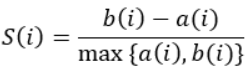
- S(i) is the silhouette coefficient of the data point i.
- a(i) is the average distance between i and all the other data points in the cluster to which i belongs.
- b(i) is the average distance from i to all clusters to which i does not belong.

Source: medium

We will then calculate the average_silhouette for every k.

Then plot the graph between average_silhouette and K.
Points to Remember While Calculating Silhouette Coefficient:
- The value of the silhouette coefficient is between [-1, 1].
- A score of 1 denotes the best, meaning that the data point i is very compact within the cluster to which it belongs and far away from the other clusters.
- The worst value is -1. Values near 0 denote overlapping clusters.
Let us see the python code with the help of an example.
range_n_clusters = [2, 3, 4, 5, 6, 7, 8]
silhouette_avg = []
for num_clusters in range_n_clusters:

 # initialise kmeans
 kmeans = KMeans(n_clusters=num_clusters)
 kmeans.fit(data_frame)
 cluster_labels = kmeans.labels_

 # silhouette score
 silhouette_avg.append(silhouette_score(data_frame, cluster_labels))plt.plot(range_n_clusters,silhouette_avg,’bx-’)
plt.xlabel(‘Values of K’)
plt.ylabel(‘Silhouette score’)
plt.title(‘Silhouette analysis For Optimal k’)
plt.show()

We see that the silhouette score is maximized at k = 3. So, we will take 3 clusters.
NOTE: The silhouette Method is used in combination with the Elbow Method for a more confident decision.
What Is Hierarchical Clustering?
In k-means clustering, the number of clusters that you want to divide your data points into, i.e., the value of K has to be pre-determined, whereas in Hierarchical clustering, data is automatically formed into a tree shape form (dendrogram).
So how do we decide which clustering to select? We choose either of them depending on our problem statement and business requirement.
Hierarchical clustering gives you a deep insight into each step of converging different clusters and creates a dendrogram. It helps you to figure out which cluster combination makes more sense. The probabilistic models that identify the probability of having clusters in the overall population are considered mixture models. K-means is a fast and simple clustering method, but it can sometimes not capture inherent heterogeneity. K-means is simple and efficient, it is also used for image segmentation, and it gives good results for much more complex deep neural network algorithms.
Conclusion
The K-means clustering algorithm is an unsupervised algorithm that is used to find clusters that have not been labeled in the dataset. This can be used to confirm business assumptions about what types of groups exist or to identify unknown groups in complex data sets. In this tutorial, we learned about how to find optimal numbers of clusters.
Key Takeaways
- With clustering, data scientists can discover intrinsic grouping among unlabelled data.
- K-means is mostly used in the fields of customer insight, marketing, medical, and social media.
Frequently Asked Questions
A. The silhouette coefficient may provide a more objective means to determine the optimal number of clusters. This is done by simply calculating the silhouette coefficient over a range of k, & identifying the peak as optimum K.
A. The optimal number of clusters k is one that maximizes the average silhouette over a range of possible values for k. Optimal of 2 clusters.
A. Optimal Value of K is usually found by square root N where N is the total number of samples.


