This article was published as a part of the Data Science Blogathon.
Introduction
This article would cover Maximal- Margin Classifier, Support Vector Classifier, and Support Vector Machines. Although many people mix these terms up, there is a significant difference between them. Let’s take a look at each one individually.
Before get going, let’s understand the hyperplane.
Hyperplane
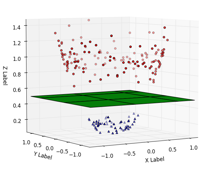
A hyperplane divides any ‘d’ dimensional space into two parts using a (d-1) dimensional hyperplane. The “green” colored 2-dimensional hyperplane is used to separate the two classes “red” and “blue” present in the third dimension, as shown in the diagram below.
 src:
src: Note!!
The data in the d dimension is divided into two parts using a (d-1) dimension hyperplane.
For instance, a point in (0-D) divides a line (in 1-D) into two parts, a line in (1-D) divides a plane (in 2-D) into two parts, and a plane (in 2-D) divides a three-dimensional space into two parts.
1. Maximal Margin Classifier
This classifier is designed specifically for linearly separable data, refers to the condition in which data can be separated linearly using a hyperplane. But, what is linearly separable data?
Linearly separable and non-linearly separable data
Linear and non-linear separable data are described in the diagram below. Linearly separable data is data that is populated in such a way that it can be easily classified with a straight line or a hyperplane. Non-linearly separable data, on the other hand, is described as data that cannot be separated using a simple straight line (requires a complex classifier).

src:https://images.app.goo.gl/qRCGETeuRa7TR9USA
However, as shown in the diagram below, there can be an infinite number of hyperplanes that will classify the linearly separable classes.
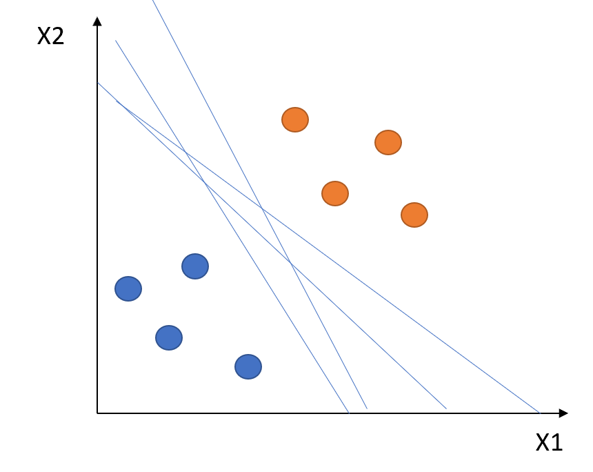
How do we choose the hyperplane that we really need?
Based on the maximum margin, the Maximal-Margin Classifier chooses the optimal hyperplane. The dotted lines, parallel to the hyperplane in the following diagram are the margins and the distance between both these dotted lines (Margins) is the Maximum Margin.
A margin passes through the nearest points from each class; to the hyperplane. The angle between these nearest points and the hyperplane is 90°. These points are referred to as “Support Vectors”. Support vectors are shown by circles in the diagram below.
This classifier would choose the hyperplane with the maximum margin which is why it is known as Maximal – Margin Classifier.

src: https://images.app.goo.gl/22RRfL4y3CUTPrxi8
Drawbacks:
This classifier is heavily reliant on the support vector and changes as support vectors change. As a result, they tend to overfit.
They can’t be used for data that isn’t linearly separable. Since the majority of real-world data is non-linear. As a result, this classifier is inefficient.
The maximum margin classifier is also known as a “Hard Margin Classifier” because it prevents misclassification and ensures that no point crosses the margin. It tends to overfit due to the hard margin. An extension of the Maximal Margin Classifier, “Support Vector Classifier” was introduced to address the problem associated with it.
2. Support Vector Classifier
Support Vector Classifier is an extension of the Maximal Margin Classifier. It is less sensitive to individual data. Since it allows certain data to be misclassified, it’s also known as the “Soft Margin Classifier”. It creates a budget under which the misclassification allowance is granted.
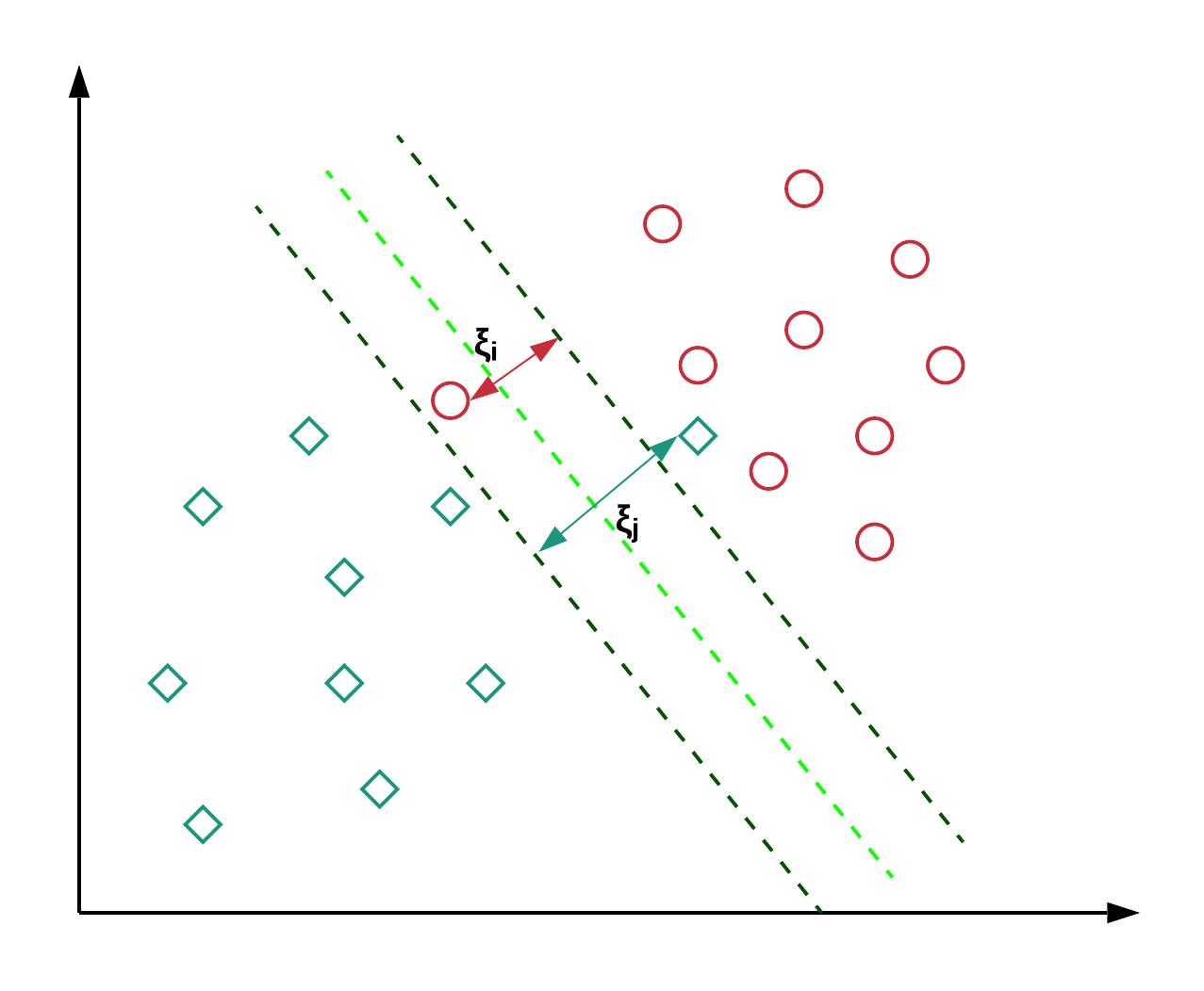
Also, It allows some points to be misclassified, as shown in the following diagram. The points inside the margin and on the margin are referred to as “Support Vectors” in this scenario. Whereas, the points on the margins were referred to as “Support vectors” in the Maximal – Margin Classifier.
src: https://images.app.goo.gl/oQ9SnHKmXVAE6Kgv6
The margin widens as the budget for misclassification increases, while the margin narrows as the budget decreases.
While building the model, we use a hyperparameter called “Cost”. Here Cost is inverse of budget means when the budget increases —> Cost decreases and vice versa. It is denoted by “C”.
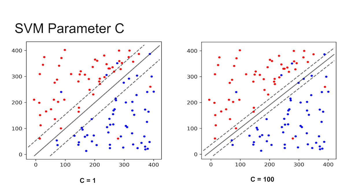
The influence of C’s value on the margin is depicted in the diagram below. When the value is small, for example, C=1, the margin widens, while when the value is high, the margin narrows down.
src: https://images.app.goo.gl/kQsSdCETBMEj2xdT8
Small ‘C’ Value —-> Large Budget —–> Wide Margin ——> Allows more misclassification
Large ‘C’ Value —-> Small Budget —–> Narrow Margin ——> Allows less misclassification
Drawback:
Only linear classification can be done by this classifier. It becomes inefficient when classification is nonlinear.
Note the difference!!!!
Maximal Margin Classifier —————————> Hard Margin Classifier
Support Vector Classifier —————————–> Soft Margin Classifier
However, all Maximum-Margin Classifiers and Support Vector Classifiers are restricted to data that can be separated linearly.
3. Support Vector Machines
Support Vector Machines are an extension of Soft Margin Classifier. It can also be used for nonlinear classification by using the kernel. As a result, this algorithm performs well in the majority of real-world problem statements. Since, in the real world, we will mostly find non-linear separable data, which will necessitate the use of complex classifiers to classify them.
Kernel: It transforms non-linear separable data from lower to higher dimensions to facilitate linear classification, as illustrated in the figure below. We use the kernel-based technique to separate non-linear data because separation can be simpler in higher dimensions.
The kernel transforms the data from lower to higher dimensions using mathematical formulas.

src: https://images.app.goo.gl/BTmyZ9RzUeWaVthT7
Understand the working of Kernel using another example
Assume, we want our model to distinguish mangoes and guavas on the x-axis, as seen in the diagram below. Our model is unable to separate them using a specific “point” on the x-axis that can differentiate both of these classes since such a point is not present here.
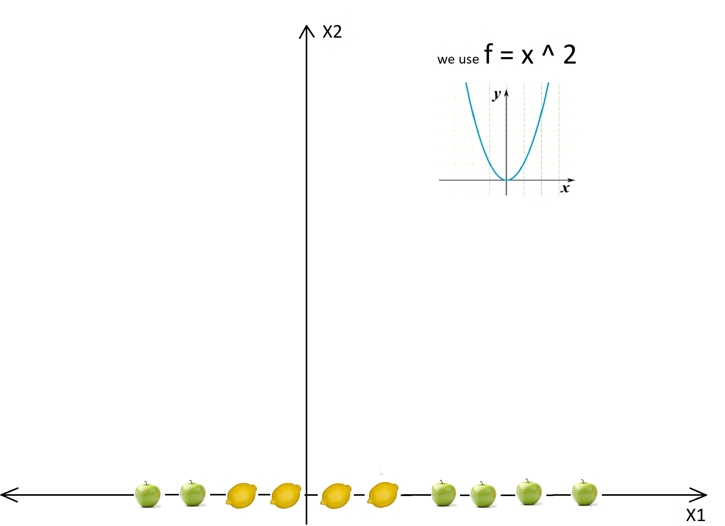
src: https://images.app.goo.gl/iMM48C6a88K8qxSw9
In this case, the kernel will transform the data populated on the x-axis using the mathematical function “f = x ^ 2″. This function will transform the straight line into a parabola where the classification is linear and relatively easier using the hyperplane.
The diagram below illustrates how a classification that was difficult in a straight line became much simpler when transformed into a parabola.
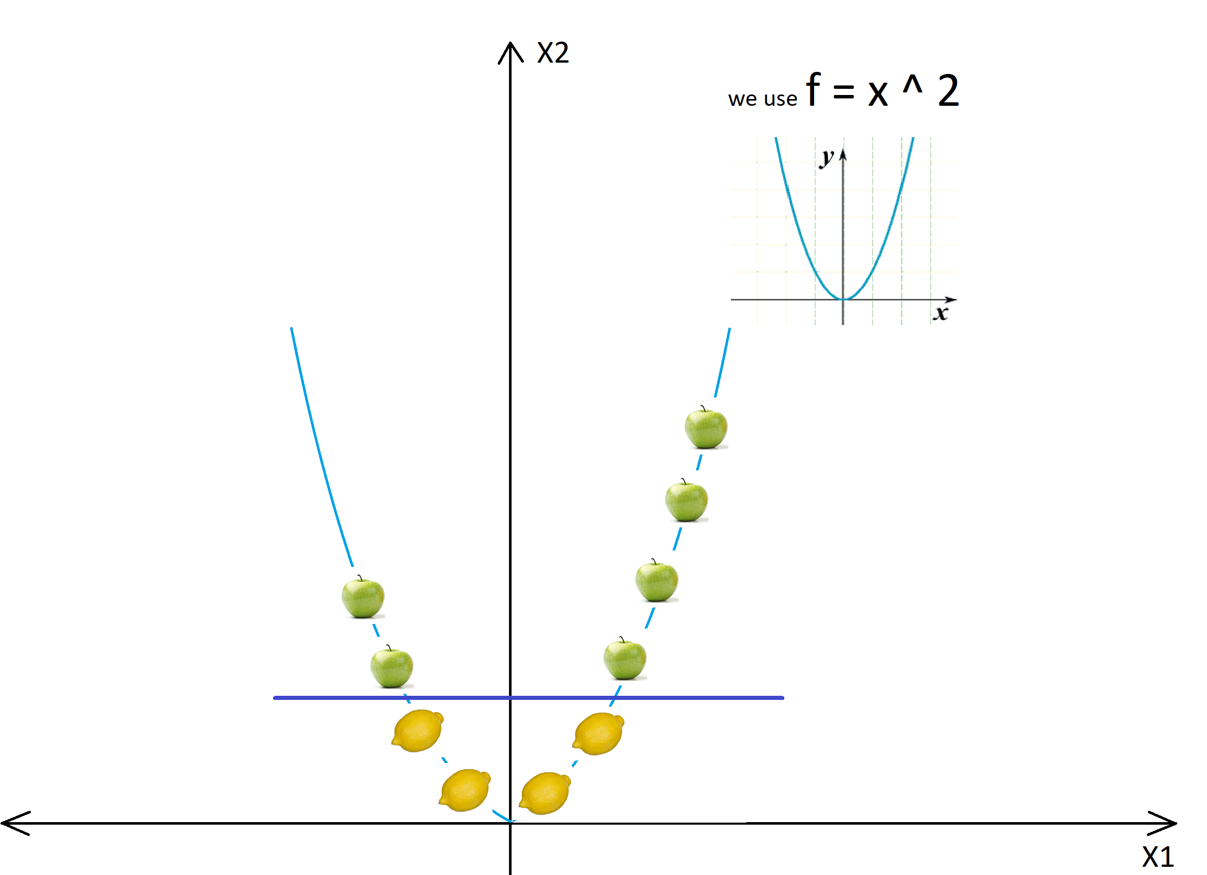
src: https://images.app.goo.gl/myBkxTcKY75vDuao9
Likewise, Kernel will apply the requisite mathematical formula to transform data into the higher dimensions, making classification in non-linearly separable data easier.
Listed below are a few SVM Kernels.
Linear Kernel = F(x, y) = sum( x.y)
Here, x, y represents the data you’re trying to classify.
The linear kernel is equivalent to the Support Vector Classifier.
Polynomial Kernel= F(x, y) = (x.y+1)^d
It is better than the Linear Kernel. Here d denotes the degree of the polynomial.
Radial Kernel= F(x, y) = exp (-gamma * ||x – y||^2)
It is highly recommended for classifying non-linear data.
The radius of impact for each point is defined by the gamma value. Where a high gamma value corresponds to a small radius of influence for each data and a low gamma value corresponds to a wide radius of influence for each data.
Understand with code in R
Step 1:
Using the library() function, load the libraries “caTools,” “e1071,” and “caret.” If these libraries aren’t already installed, use install.pacakges() to do so.
library(caTools)
library(e1071)
library(caret)
Step 2:
Now, load the data set into the ‘data’ variable; in this case, we are using diabetes data with the attributes “Pregnancies,” “Glucose,” “BloodPressure,” “SkinThickness,” “Insulin,” “BMI,” “DiabetesPedigreeFunction,” “Age,” and “Outcome.” The response variable is “Outcome” in this case.
After loading the data, split it into two parts: train and test. We used 70% of the data for training and 30% for testing.
data<- read.csv(diabetes.csv, header=T)
set.seed(123)
split <- sample.split(data,SplitRatio = 0.7)
train <- subset(data,split==T)
test <- subset(data,split==F)
Step 3:
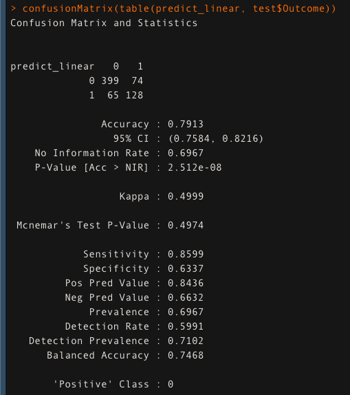
To begin, I built the model using the linear kernel. The Cost parameter’s hyperparameter tuning was also done
The model has an accuracy of 79.13 % on the test data while using the linear kernel.
set.seed(123)
hypertunelinear <- tune(svm,Outcome~., data = train, kernel="linear", ranges = list(cost=c(0.1,0.5,1, 1.5, 2,10)))
Linearmodel <- hypertunelinear$best.model
###predict using linear kernel
predict_linear <- predict(Linearmodel,test)
confusionMatrix(table(predict_linear, test$Outcome))
Step 4:
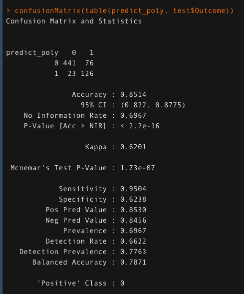
Thereafter, I used the polynomial kernel with the hyperparameter tuning of Cost and degree parameters. The model built using the polynomial kernel is giving an accuracy of “85.14%“
set.seed(123)
hypertune_Poly <- tune(svm,Outcome~., data = train,cross=4, kernel="polynomial", ranges = list(cost=c(0.1,0.5,1, 1.5, 2,10), degree=c(0.5,1,2,3,4)))
polynomial_model <- hypertune_Poly$best.model
##predict using polynomial kernel
predict_poly <- predict(polynomial_model, test)
confusionMatrix(table(predict_poly, test$Outcome))
Step 5:
Finally, the model was built using the radial kernel. Here, the hyperparameters “cost” and “gamma” are tuned. Of all the models built so far, it has the highest accuracy. The accuracy of the model built using radial kernel is “98.2%”
set.seed(123)
hypertune_radial <- tune(svm,Outcome~., data = train,cross=4, kernel="radial", ranges = list(cost=c(0.1,0.5,1, 1.5, 2,10),gamma=c(0.01,0.1,0.5,1,2,3)))
radial_model <- hypertune_radial$best.model
##predict using radial kernel
predict_radial <- predict(radial_model, test)
confusionMatrix(table(predict_radial, test$Outcome))
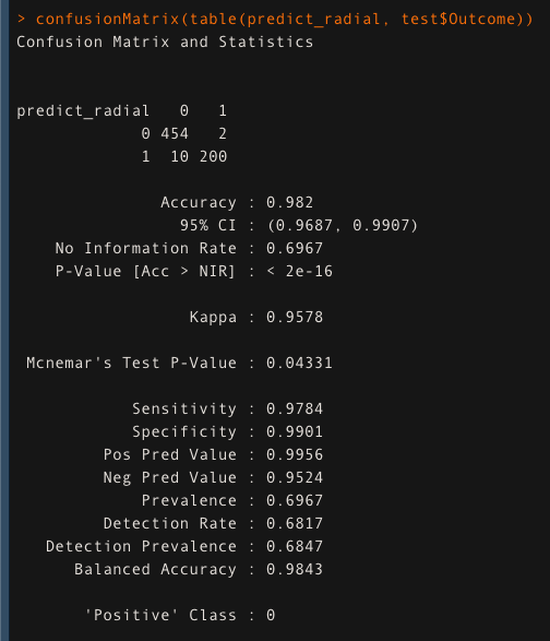
In this case, the radial kernel model outperforms the polynomial and linear kernel models in terms of accuracy. However, this is not always the case. If the data is linearly separable, the linear kernel would outperform the polynomial and radial kernels significantly.
Thank you,
Shivam Sharma.
Phone: +91 7974280920
E-Mail: [email protected]
LinkedIn: www.linkedin.com/in/shivam-sharma-49ba71183
The media shown in this article are not owned by Analytics Vidhya and is used at the Author’s discretion.
Shivam Sharma
26 Oct, 2021


