Beginner’s Guide to Universal Approximation Theorem
Introduction
Neural networks are used for so many tasks in the fields of machine learning and deep learning. This, however, begs the question- why are they so powerful?
This article puts forth one explanation – the universal approximation theorem.
Let’s start with defining what it is. In simple words, the universal approximation theorem says that neural networks can approximate any function. Now, this is powerful. Because, what this means is that any task that can be thought of as a function computation, can be performed/computed by the neural networks. And almost any task that neural network does today is a function computation – be it language translation, caption generation, speech to text, etc. If you ask, how many layers will be required for any function computation? The answer is only 1.
In this article, we will try and understand why the theorem is true.
WORD OF CAUTION
There are two important facts to be noted.
1. It is important to realize that the word used is approximate. This means that the function computed is not exact. However, this approximation can be improved as the number of computation units i.e. neurons are increased in the layer and it can be fit to the desired accuracy.
2. The function we compute this way are continuous functions. The generality does not hold for discontinuous functions. However, more often than not, continuous functions prove to be a good enough substitute for discontinuous functions, and therefore, the neural networks can work.
Therefore, let’s go ahead and understand this very important theorem. Before jumping to the visual proof though, let us have a look at a perceptron – the basic unit of computation.
PERCEPTRON
A perceptron can be understood as the basic computation unit of neural networks.
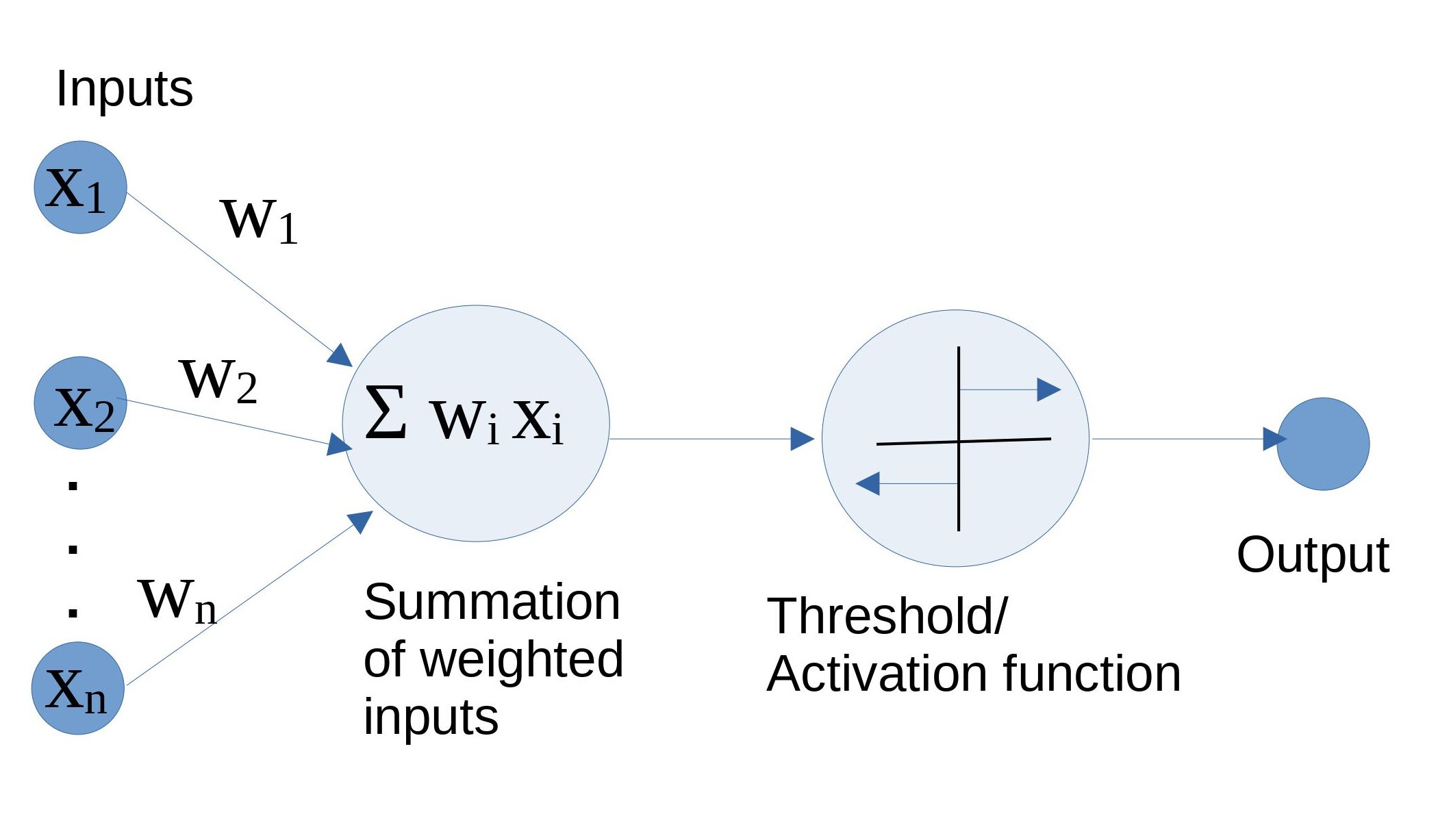
Figure 1: The perceptron, in its mathematical glory Referenced image: Slide 7, from the presentation titled Neural Networks: What can a network represent; URL in the reference list, numbered 3
In the above diagram, inputs xi through xn is multiplied with their respective weights wi through wn . This is what forms the weighted inputs which are then summed up (Σ wi xi). Next, this sum passes through a threshold/activation function which functions as an on/off switch. It allows the neuron to fire if the value of the sum is greater than a certain threshold otherwise the input is inhibited. This is the final value that constitutes the output. Activation functions are also the magical ingredient of non-linearity without which, a perceptron and eventually, the neural network would just be a linear combination of inputs. We will use the activation function sigmoid to understand the basics.
CONVERTING SIGMOID TO STEP FUNCTION
We intend to output 1 for inputs greater than a threshold and 0 for inputs less than the threshold. A sigmoid function does exactly that.
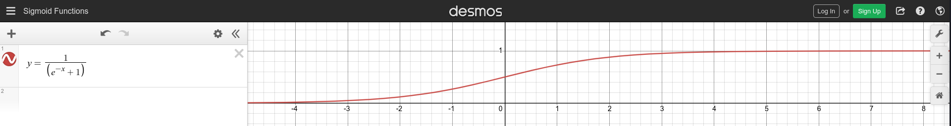
Figure 2: The sigmoid function. Graph made using the desmos tool.
But, there’s a problem- the slope of the sigmoid function. In the output layer, we intend to add up outputs of hidden layer neurons. It will be easier to work with adding integers directly than adding the real numbered outputs of the sigmoid function. Therefore, we will need a step function. Turns out, when applied enough weight, the sigmoid function can be tuned to behave just like a step function. So, to make our lives easier, we will do just that.
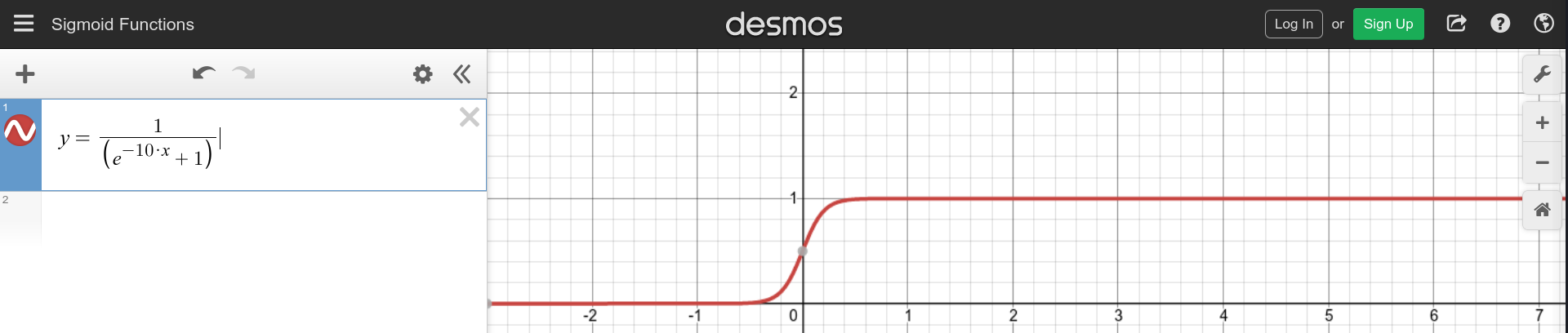
Figure 3.1: The sigmoid function with weight 10. Graph made using the desmos tool.

Figure 3.2: The sigmoid function with weight 100. Graph made using the desmos tool.
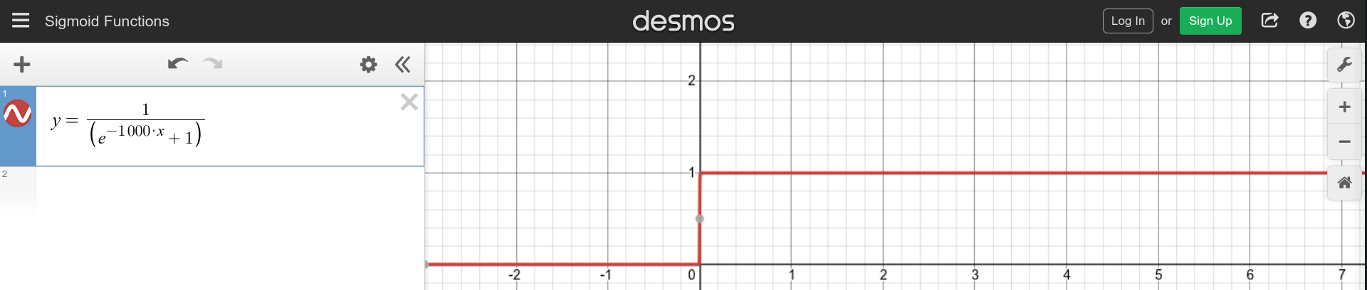
Figure 3.3: The sigmoid function with weight 1000. Graph made using the desmos tool.
The weight 1000 seems a good choice. Adding the bias will help shift the curve to the value of x we intend. Since, we have confirmed for ourselves, from here on in the article, we will treat the outputs from individual neurons in the hidden layer as if by a step function.
USING PERCEPTRON FOR UNDERSTANDING THE PROOF
Let’s start computing functions with a single perceptron in the hidden layer ( hidden layers are the layers except for the input and output layers ).
Let us plot a boolean AND function just to try (it is not related to proof). Both the domain and range of this function are the boolean values {0,1}. In the output ( the bigger circle) the inputs are getting added. This neuron will fire only if both the inputs it receives are 1 otherwise it won’t. By firing, we mean the output is 1, and by not firing we mean, the output is 0.
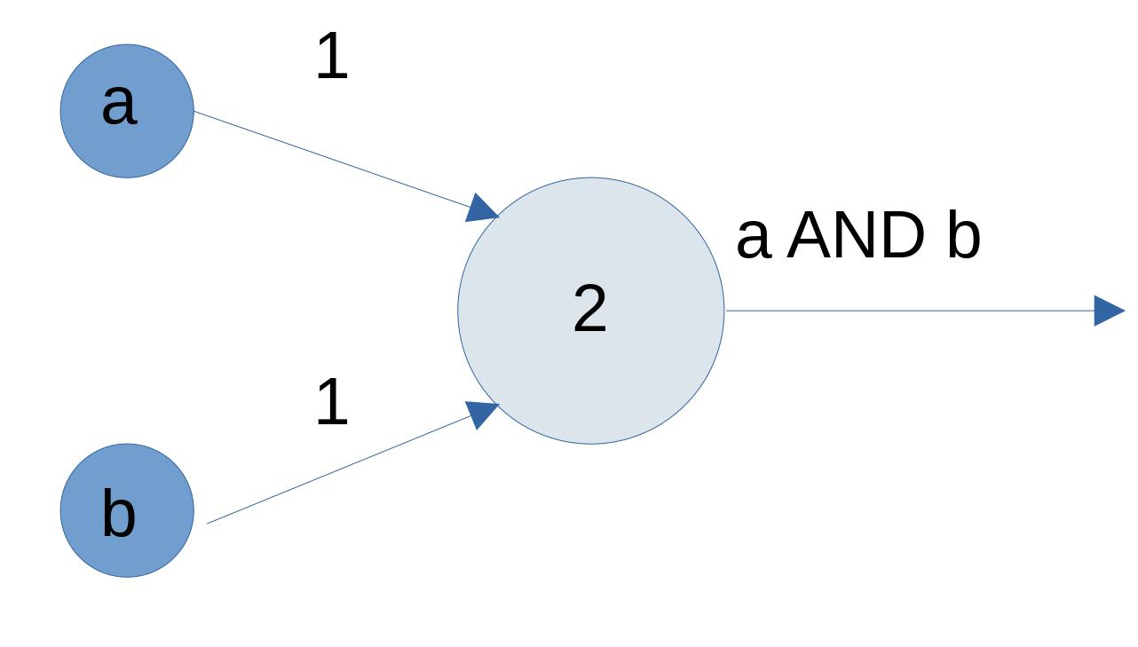
Figure 4: Boolean AND function using perceptron Referenced image: Slide 21, from the presentation titled Neural Networks: What can a network represent; URL in the reference list, numbered 3
So, we know how to plot a function. Moving on, let us plot a function using perceptron which outputs 1 on the input being greater than a threshold value T1 and 0 on being less than that. As described in the cases of the previous section, we will have to assign a high weight value and a bias T1 to get the following graph.
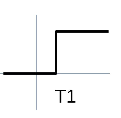
Figure 5: Threshold activation. Referenced image: Chapter 4, A visual proof that neural nets can compute any function, Michael Nilson; URL in the reference list, numbered 1
Since we have brushed up the basics, let’s move on to understanding the visual proof of the universal approximation theorem. This proof follows closely the visual proof provided by Michael Nilson in his textbook on Neural networks, the link to which is provided in the references section.
What if we want to plot the function wherein 1 is output only when the input value lies between T1 and T2 and in all other cases, the value that is output is 0? For accomplishing this, we will need two perceptrons accepting the same input but with different thresholds as shown here. The network of 2 perceptrons forms an MLP – multi-layer perceptron. Note that the output layer has additive activation yet.
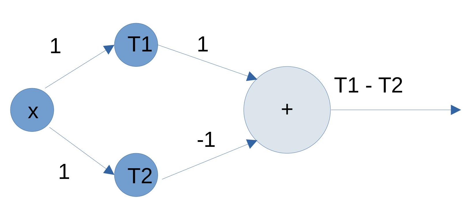
Figure 6.1: perceptron network for building a rectangle Referenced image: Slide 117, from the presentation titled Neural Networks: What can a network represent; URL in the reference list, numbered 3
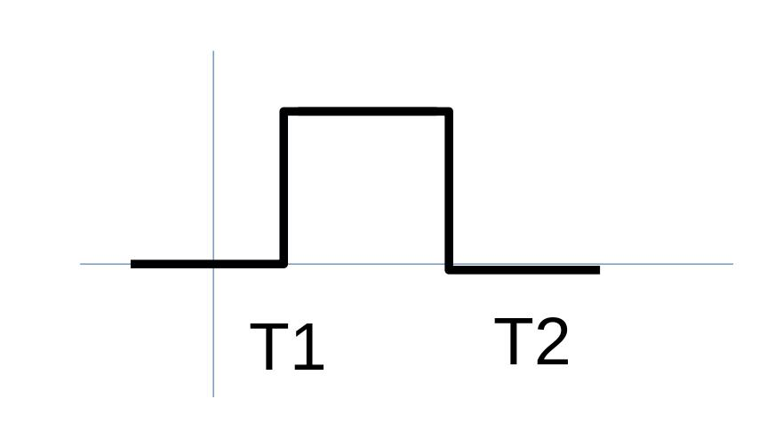
Figure 6.2: Graph corresponding to the network in figure 6.1. Referenced image: Slide 117, from the presentation titled Neural Networks: What can a network represent; URL in the reference list, numbered 3
This graph seems like a rectangle. In the face of a continuous function, many rectangles like this can be combined of varying heights to suit the boundary of the function. In terms of architecture, several perceptrons can be stacked together to achieve this function.
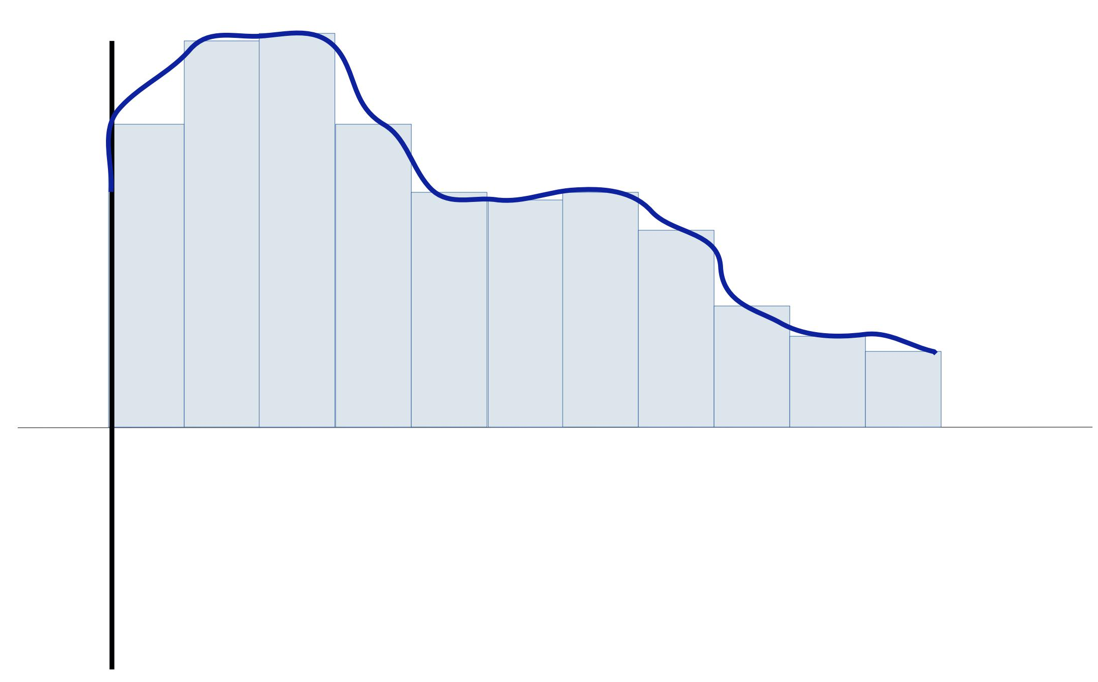
Figure 7: Putting together the rectangles. Referenced image: Slide 118, from the presentation titled Neural Networks: What can a network represent; URL in the reference list, numbered 3
This is the approximation of the function we were talking about.
But wait, whatever we have seen till now is only the combination of weighted inputs. We never passed it through the sigmoid function of the final neuron (In the above image, the bigger circle has addition as its function and is never followed by sigmoid). So? It’s easy. Assuming the bias of the final output neuron is 0, we need this hidden layer to calculate σ -1 of the original function. The inverse of a function gives the original value for which the function gave an output. Or in other words, the important property of inverses is:
f(g(x)) = g(f(x)) = x where f(x) is inverse of g(x) ( also denoted by g-1(x) ).
Therefore, σ -1( σ(y) ) = σ ( σ-1(y) ) = y where y is the original function we intend to compute.
So the hidden layers instead compute the inverted function and the final activation inverts it back to the original. The inverted function is still a function and can be approximated using the idea of rectangles described above.
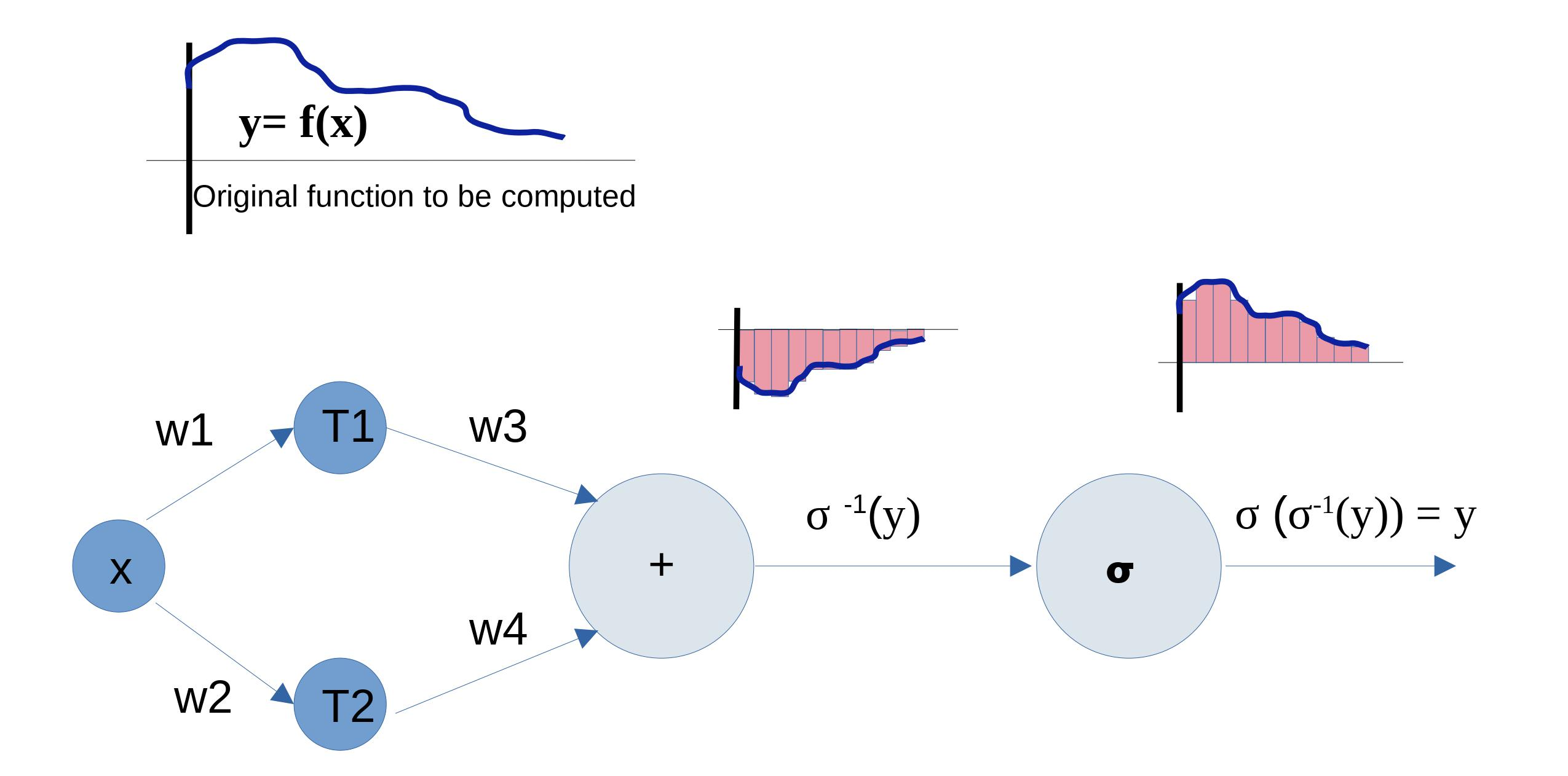
Figure 8: The big picture. Image by the author
For any continuous function, this approach can be adopted. All the stacked perceptrons form, however, only a single layer in the neural network. The purpose is achieved!
What if we want to increase the precision. Simple – we decrease the width of the rectangles. In terms of terminology already established, we make | T2 – T1 |< ε, where ε denotes the precision we desire and | T2 – T1 | is the width of the rectangle.
Thus, we establish a visual proof to the universal approximation theorem in two dimensions. This proof stands true for the higher dimensions too, wherein visualization becomes difficult but the concept remains the same.
REFERENCES
These are some of the awesome places to learn more about this topic. Do visit them!
- Visual Proof by Michael Nilson: http://neuralnetworksanddeeplearning.com/chap4.html
- CMU Lecture 2: The Universal Approximation Theorem: https://www.youtube.com/watch?v=lkha188L4Gs
- Slides: https://www.cs.cmu.edu/~bhiksha/courses/deeplearning/Fall.2019/www.f19/document/lecture/lecture-2.pdf


