img src: https://wallpapercave.com/w/wp7461543
Introduction
The major objective of watching or reading news was to be informed about whatever is happening around us. There are several social media platforms in the current modern era, like Facebook, Twitter, Reddit, and so forth where millions of users would rely upon for knowing day-to-day happenings. Then came the fake news which spread across people as fast as the real news could. Fake news is a piece of incorporated or falsified information often aimed at misleading people to a wrong path or damage a person or an entity’s reputation.
Characteristics of Fake News:
- Their sources are not genuine.
- May or may not have grammatical errors.
- Often uses attention-seeking words, click baits, etc.
- Seems too good to be true.
- Mimics the real headlines and twists the story.
A study shows that a fake tweet on Twitter spreads six times faster than the real one. Thus, it becomes necessary to find whether a piece of news is true or fake whenever we read any information on the web.
As humans, when we read an article, we could somehow understand its context by interpreting its words. Given today’s volume of news, it is possible to teach computers how to read and understand the difference between real and fake news using NLP techniques. All you need here are the appropriate Machine Learning algorithms and a dataset.
Let’s have a quick look at the workflow for the Fake news classifier model!
1.Data Collection:
The process of gathering information from various and all possible resources regarding a particular research problem. This information is stored in a file as the dataset and is subject to various techniques like testing, evaluation, etc.
2.Data Cleaning:
Identification and removal of errors if any in the gathered information. This process is carried out mainly to improve the dataset’s quality, make it reliable, and provide accurate decision-making processes.
3.Data Exploration/Analysis:
Various visualization techniques are carried out here to understand the dataset in terms of its characteristics namely, size, quantity, etc. This process is essential to better understand the nature of the dataset and get insights faster.
4.Data Modelling:
The process of training the dataset using one or more ML algorithms to tune it according to the business need, predict or validate it accordingly.
5.Data Validation:
The method of tuning the hyperparameters before testing the model. This provides an unbiased evaluation of a model fit done on the training dataset.
6.Deployment:
Integrating an ML model into an existing environment to make more practical business decisions based on the dataset.

img src: https://wallpapercave.com/w/wp7461541
Python Implementation
The dataset downloaded from Kaggle has the following attributes: Id, Title, Author, Text, and the Label (where 1 is unreliable and 0 is reliable).
import pandas as pd
df = pd.read_csv('news.csv')
#df.head()
Having downloaded and read the dataset, we now have to check and classify its features (or attributes), this step generally depends on what the dataset contains and what we are about to analyze. Thus, in this classifier model, we’ll be taking the “Id”, “Title” and “Author” columns as Independent features and the “Label” column as a dependent feature.
#get the independent features
X = df.drop('label',axis =1)
#X.head()
#get dependent variables
y = df['label']
#y.head()
In total, there are about 20800 records.
df.shape
Output:
(20800, 5)
The dataset is checked for any missing values and those are dropped.
from sklearn.feature_extraction.text import CountVectorizer,TfidfVectorizer,HashingVectorizer
df = df.dropna()
#df.head(10)
Now we’ll create a copy of this dataset and also reset its index values.
messages = df.copy()
messages.reset_index(inplace = True)
#messages.head(10)
This part of the code is for Stopword removal and Stemming. Here, the corpus is an array in which we have appended all the titles of the news.
import re
from nltk.corpus import stopwords
from nltk.stem.porter import PorterStemmer
ps = PorterStemmer()
corpus = []
for i in range(0, len(messages)):
    review = re.sub('[^a-zA-Z]', ' ', messages['title'][i])
    review = review.lower()
    review = review.split()
    review = [ps.stem(word) for word in review if not word in stopwords.words('english')]
    review = ' '.join(review)
    corpus.append(review)
#corpus[3]
Applying count vectorizer (also known as the “Bag of Words”). Maximum features passed here are 5000.
#Applying countvectorizer
#Creating the bag of words model
from sklearn.feature_extraction.text import CountVectorizer
cv = CountVectorizer(max_features = 5000,ngram_range=(1,3))
X = cv.fit_transform(corpus).toarray()
X.shape #(18285, 5000)
y =messages['label']
Dataset is now split into train and test. The first 20 features are displayed here.
#Divide the dataset into train and test
from sklearn.model_selection import train_test_split
X_train,X_test,y_train,y_test = train_test_split(X,y,test_size = 0.33,random_state = 0)
cv.get_feature_names()[:20]
Output:
[‘abandon’,
‘abc’,
‘abc news’,
‘abduct’,
‘abe’,
‘abedin’,
‘abl’,
‘abort’,
‘abroad’,
‘absolut’,
‘abstain’,
‘absurd’,
‘abus’,
‘abus new’,
‘abus new york’,
‘academi’,
‘accept’,
‘access’,
‘access pipelin’,
‘access pipelin protest’]
We’ll now get the parameters as the next step.
cv.get_params()
Output:
{‘analyzer’: ‘word’,
‘binary’: False,
‘decode_error’: ‘strict’,
‘dtype’: numpy.int64,
‘encoding’: ‘utf-8’,
‘input’: ‘content’,
‘lowercase’: True,
‘max_df’: 1.0,
‘max_features’: 5000,
‘min_df’: 1,
‘ngram_range’: (1, 3),
‘preprocessor’: None,
‘stop_words’: None,
‘strip_accents’: None,
‘token_pattern’: ‘(?u)\b\w\w+\b’,
‘tokenizer’: None,
‘vocabulary’: None}
The array is converted into dataframe.
count_df = pd.DataFrame(X_train,columns = cv.get_feature_names())
#count_df.head()
Using the matplotlib function, lets plot a confusion matrix. This part of the code and the plot_confusion_matrix function will be used in all the upcoming algorithms for its training and accuracy prediction purpose.
import matplotlib.pyplot as plt
def plot_confusion_matrix(cm, classes,
                          normalize=False,
                          title='Confusion matrix',
                          cmap=plt.cm.Blues):
    plt.imshow(cm, interpolation='nearest', cmap=cmap)
    plt.title(title)
    plt.colorbar()
    tick_marks = np.arange(len(classes))
    plt.xticks(tick_marks, classes, rotation=45)
    plt.yticks(tick_marks, classes)
if normalize:
        cm = cm.astype('float') / cm.sum(axis=1)[:, np.newaxis]
        print("Normalized confusion matrix")
    else:
        print('Confusion matrix, without normalization')
thresh = cm.max() / 2.
    for i, j in itertools.product(range(cm.shape[0]), range(cm.shape[1])):
        plt.text(j, i, cm[i, j],
                 horizontalalignment="center",
                 color="white" if cm[i, j] > thresh else "black")
plt.tight_layout()
    plt.ylabel('True label')
    plt.xlabel('Predicted label')
Multinomial Naive Bayes Algorithm
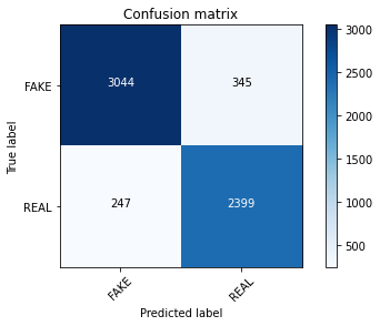
This algorithm considers the integer feature counts where it represents how often or how many times a specific word appears. It is much suitable for the classification of discrete features. i.e. word counts for classifying a text. The Prediction Accuracy we’ve got here is 90%.
from sklearn.naive_bayes import MultinomialNB
classifier = MultinomialNB()
from sklearn import metrics
import numpy as np
import itertools
classifier.fit(X_train,y_train)
pred = classifier.predict(X_test)
score = metrics.accuracy_score(y_test,pred)
print("Accuracy: %0.3f"%score)
cm = metrics.confusion_matrix(y_test,pred)
plot_confusion_matrix(cm, classes=['FAKE', 'REAL'])
Output:
Accuracy: 0.902
Confusion matrix, without normalization

classifier.fit(X_train, y_train)
pred = classifier.predict(X_test)
score = metrics.accuracy_score(y_test, pred)
score
Output:
0.9019055509527755
y_train.shape #(12250,)
pred #array([1, 1, 1, ..., 0, 0, 1])
Passive Aggressive Classifier Algorithm
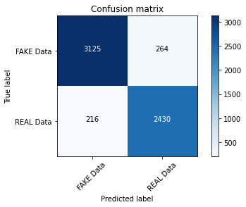
The PAC algorithm responds aggressively to incorrect predictions and remains passive for the correct predictions. By using this algorithm, the accuracy is 92%.
from sklearn.linear_model import PassiveAggressiveClassifier
linear_clf = PassiveAggressiveClassifier(max_iter=50)
linear_clf.fit(X_train,y_train)
pred = linear_clf.predict(X_test)
score = metrics.accuracy_score(y_test,pred)
print("Accuracy: %0.3f"%score)
cm = metrics.confusion_matrix(y_test,pred)
plot_confusion_matrix(cm,classes = ['FAKE Data','REAL Data'])
Output:
Accuracy: 0.920
Confusion matrix, without normalization

Multinomial Classifier with Hyperparameter (alpha)
It’s none other than the Multinomial Naive Bayes algorithm we trained earlier but here we’ll be adding a hyperparameter for it and for each alpha value, the corresponding scores are calculated. At alpha = 0.3, the score seems to be maximum.
The more negative the coefficient value, the word is used in fake news!
classifier=MultinomialNB(alpha=0.1)
previous_score=0
for alpha in np.arange(0,1,0.1):
    sub_classifier=MultinomialNB(alpha=alpha)
    sub_classifier.fit(X_train,y_train)
    y_pred=sub_classifier.predict(X_test)
    score = metrics.accuracy_score(y_test, y_pred)
    if score>previous_score:
        classifier=sub_classifier
    print("Alpha: {}, Score : {}".format(alpha,score))
Output:
Alpha: 0.0, Score : 0.8903065451532726
Alpha: 0.1, Score : 0.9020712510356255
Alpha: 0.2, Score : 0.9025683512841757
Alpha: 0.30000000000000004, Score : 0.9024026512013256
Alpha: 0.4, Score : 0.9017398508699255
Alpha: 0.5, Score : 0.9015741507870754
Alpha: 0.6000000000000001, Score : 0.9022369511184756
Alpha: 0.7000000000000001, Score : 0.9025683512841757
Alpha: 0.8, Score : 0.9015741507870754
Alpha: 0.9, Score : 0.9017398508699255
#get features names
feature_names = cv.get_feature_names()
classifier.coef_[0]
Output:
array([ -9.10038883, -8.62276128, -9.10038883, …,
–10.79498456, -8.91467169, -9.32864749])
And yay! Here you can see we have classified the most real and most fake news based on their coefficients. The fake news classifier model we just implemented has worked out pretty well 😀
#Most real
sorted(zip(classifier.coef_[0], feature_names), reverse=True)[:20]
Output:
[(-4.000149156604985, ‘trump’),
(-4.287872694443541, ‘hillari’),
(-4.396389621061519, ‘clinton’),
(-4.899969726208735, ‘elect’),
(-5.176598600897756, ‘new’),
(-5.234730366348767, ‘comment’),
(-5.273968180973631, ‘video’),
(-5.3868167681180115, ‘war’),
(-5.396821854078974, ‘us’),
(-5.412019714988405, ‘hillari clinton’),
(-5.417137433425386, ‘fbi’),
(-5.48068448454208, ‘vote’),
(-5.566255475855405, ’email’),
(-5.578238842742501, ‘world’),
(-5.634015380199913, ‘obama’),
(-5.734501455772904, ‘donald’),
(-5.763095255139644, ‘donald trump’),
(-5.785090276725191, ‘russia’),
(-5.846224665218559, ‘day’),
(-5.862110622807369, ‘america’)]
#Most fake
sorted(zip(classifier.coef_[0], feature_names))[:20]
Output:
[(-10.794984555596727, ‘abe’),
(-10.794984555596727, ‘abroad’),
(-10.794984555596727, ‘abus new’),
(-10.794984555596727, ‘abus new york’),
(-10.794984555596727, ‘act new’),
(-10.794984555596727, ‘act new york’),
(-10.794984555596727, ‘advic’),
(-10.794984555596727, ‘advis new’),
(-10.794984555596727, ‘advis new york’),
(-10.794984555596727, ‘age new’),
(-10.794984555596727, ‘age new york’),
(-10.794984555596727, ‘agenda breitbart’),
(-10.794984555596727, ‘ail’),
(-10.794984555596727, ‘aleppo new’),
(-10.794984555596727, ‘aleppo new york’),
(-10.794984555596727, ‘ali’),
(-10.794984555596727, ‘america breitbart’),
(-10.794984555596727, ‘america new york’),
(-10.794984555596727, ‘american breitbart’),
(-10.794984555596727, ‘american new’)]
If you’re an enthusiast who is looking forward to unravel the world of Generative AI. Then, please register for our upcoming event, DataHack Summit 2023.


%202.jpg)