This article was published as a part of the Data Science Blogathon
In Neural Networks, we have the concept of Loss Functions, which tells us about the performance of our neural networks i.e, at the current instant, how good or poor the model is performing. Now, to train our network such that it performs better on the unseen datasets, we need to take the help of the loss. Essentially, our objective is to minimize the loss, as lower loss implies that our model is going to perform better. So, Optimization means minimizing (or maximizing) any mathematical expression.
Optimizers are algorithms or methods used to update the parameters of the network such as weights, biases, etc to minimize the losses. Therefore, Optimizers are used to solve optimization problems by minimizing the function i.e, loss function in the case of neural networks.
So, In this article, we’re going to explore and deep dive into the world of optimizers for deep learning models. We will also discuss the foundational mathematics behind these optimizers and discuss their advantages, and disadvantages.
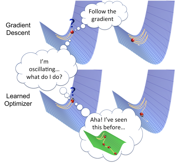
Image Source: Google Images
1. Role of an Optimizer
2. The Intuition behind Optimizers with an Example
3. Instances of Gradient Descent Optimizers
4. Challenges with all Types of Gradient-based Optimizers
As discussed in the introduction part of the article, Optimizers update the parameters of neural networks such as weights and learning rate to minimize the loss function. Here, the loss function acts as a guide to the terrain telling optimizer if it is moving in the right direction to reach the bottom of the valley, the global minimum.
Let us imagine a climber hiking down the hill with no sense of direction. He doesn’t know the right way to reach the valley in the hills, but, he can understand whether he is moving closer (going downhill) or further away (uphill) from his final destination. If he keeps taking steps in the correct direction, he will reach to his aim i.,e the valley
Exactly, this is the intuition behind optimizers- to reach a global minimum concerning the loss function.
Different instances of Gradient descent based Optimizers are as follows:
Gradient descent is an optimization algorithm that’s used when training deep learning models. It’s based on a convex function and updates its parameters iteratively to minimize a given function to its local minimum.
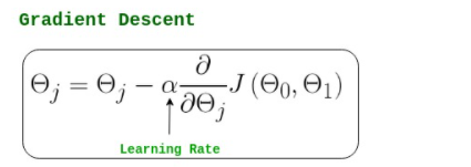
The notation used in the above Formula is given below,
In the above formula,
As you can see, the gradient represents the partial derivative of J(cost function) with respect to ϴj
Note that, as we reach closer to the global minima, the slope or the gradient of the curve becomes less and less steep, which results in a smaller value of derivative, which in turn reduces the step size or learning rate automatically.
It is the most basic but most used optimizer that directly uses the derivative of the loss function and learning rate to reduce the loss function and tries to reach the global minimum.
Thus, the Gradient Descent Optimization algorithm has many applications including-

The above-described equation calculates the gradient of the cost function J(θ) with respect to the network parameters θ for the entire training dataset:
Image Source: Google Images
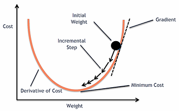
Our aim is to reach at the bottom of the graph(Cost vs weight), or to a point where we can no longer move downhill–a local minimum.
In general, Gradient represents the slope of the equation while gradients are partial derivatives and they describe the change reflected in the loss function with respect to the small change in parameters of the function. Now, this slight change in loss functions can tell us about the next step to reduce the output of the loss function.
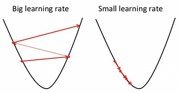
Learning rate represents the size of the steps our optimization algorithm takes to reach the global minima. To ensure that the gradient descent algorithm reaches the local minimum we must set the learning rate to an appropriate value, which is neither too low nor too high.
Taking very large steps i.e, a large value of the learning rate may skip the global minima, and the model will never reach the optimal value for the loss function. On the contrary, taking very small steps i.e, a small value of learning rate will take forever to converge.
Thus, the size of the step is also dependent on the gradient value.
Image Source: Google Images
As we discussed, the gradient represents the direction of increase. But our aim is to find the minimum point in the valley so we have to go in the opposite direction of the gradient. Therefore, we update parameters in the negative gradient direction to minimize the loss.
Algorithm: θ=θ−α⋅∇J(θ)
In code, Batch Gradient Descent looks something like this:
for x in range(epochs):
    params_gradient = find_gradient(loss_function, data, parameters)
    parameters = parameters - learning_rate * params_gradient
1. Easy computation.
2. Easy to implement.
3. Easy to understand.
1. May trap at local minima.
2. Weights are changed after calculating the gradient on the whole dataset. So, if the dataset is too large then this may take years to converge to the minima.
3. Requires large memory to calculate gradient on the whole dataset.
To overcome some of the disadvantages of the GD algorithm, the SGD algorithm comes into the picture as an extension of the Gradient Descent. One of the disadvantages of the Gradient Descent algorithm is that it requires a lot of memory to load the entire dataset at a time to compute the derivative of the loss function. So, In the SGD algorithm, we compute the derivative by taking one data point at a time i.e, tries to update the model’s parameters more frequently. Therefore, the model parameters are updated after the computation of loss on each training example.
So, let’s have a dataset that contains 1000 rows, and when we apply SGD it will update the model parameters 1000 times in one complete cycle of a dataset instead of one time as in Gradient Descent.
Algorithm: θ=θ−α⋅∇J(θ;x(i);y(i)) , where {x(i) ,y(i)} are the training examples
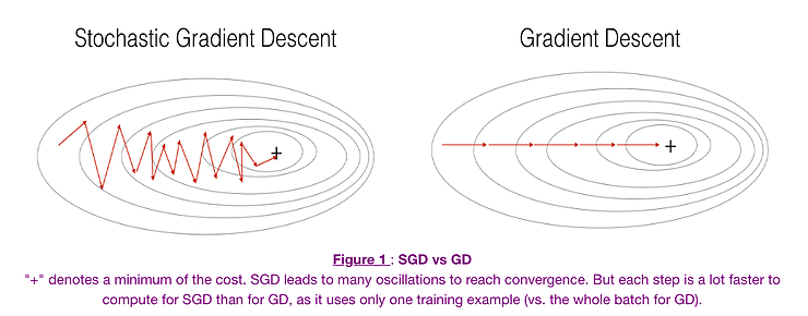
We want the training, even more, faster, so we take a Gradient Descent step for each training example. Let’s see the implications in the image below:
Image Source: Google Images
Let’s try to find some insights from the above diagram:
It is observed that in SGD the updates take more iterations compared to GD to reach minima. On the contrary, the GD takes fewer steps to reach minima but the SGD algorithm is noisier and takes more iterations as the model parameters are frequently updated parameters having high variance and fluctuations in loss functions at different values of intensities.
Its code snippet simply adds a loop over the training examples and finds the gradient with respect to each of the training examples.
for x in range(epochs):
    np.random.shuffle(data)
    for example in data:
        params_gradient = find_gradient(loss_function, example, parameters)
        parameters = parameters - learning_rate * params_gradient
1. Convergence takes less time as compared to others since there are frequent updates in model parameters.
2. Requires less memory as no need to store values of loss functions.
3. May get new minima’s.
1. High variance in model parameters.
2. Even after achieving global minima, it may overshoots.
3. To reach the same convergence as that of gradient descent, we need to slowly reduce the value of the learning rate.
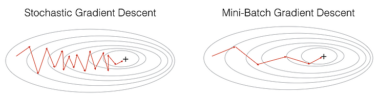
To overcome the problem of large time complexity in the case of the SGD algorithm. MB-GD algorithm comes into the picture as an extension of the SGD algorithm. It’s not all but it also overcomes the problem of Gradient descent. Therefore, It’s considered the best among all the variations of gradient descent algorithms. MB-GD algorithm takes a batch of points or subset of points from the dataset to compute derivate.
Image Source: Google Images
It is observed that the derivative of the loss function for MB-GD is almost the same as a derivate of the loss function for GD after some number of iterations. But the number of iterations to achieve minima is large for MB-GD compared to GD and the cost of computation is also large.
Therefore, the weight updation is dependent on the derivate of loss for a batch of points. The updates in the case of MB-GD are much noisy because the derivative is not always towards minima.
It updates the model parameters after every batch. So, this algorithm divides the dataset into various batches and after every batch, it updates the parameters.
Algorithm: θ=θ−α⋅∇J(θ; B(i)), where {B(i)} are the batches of training examples
In the code snippet, instead of iterating over examples, we now iterate over mini-batches of size 30:
for x in range(epochs):
    np.random.shuffle(data)
    for batch in get_batches(data, batch_size=30):
        params_gradient = find_gradient(loss_function, batch, parameters)
        parameters = parameters - learning_rate * params_gradient
1. Updates the model parameters frequently and also has less variance.
2. Requires not less or high amount of memory i.e requires a medium amount of memory.
1. The parameter updation in MB-SGD is much noisy compared to the weight updation in the GD algorithm.
2. Compared to the GD algorithm, it takes a longer time to converge.
3. May get stuck at local minima.
Choosing an optimum value of the learning rate. If we choose the learning rate as a too-small value, then gradient descent may take a very long time to converge. For more about this challenge, refer to the above section of Learning Rate which we discussed in the Gradient Descent Algorithm.
For all the parameters, they have a constant learning rate but there may be some parameters that we may not want to change at the same rate.
May get stuck at local minima i.e, not reach up to the local minimum.
Thanks for reading!
If you liked this and want to know more, go visit my other articles on Data Science and Machine Learning by clicking on the Link
Please feel free to contact me on Linkedin, Email.
Something not mentioned or want to share your thoughts? Feel free to comment below And I’ll get back to you.
Currently, I am pursuing my Bachelor of Technology (B.Tech) in Computer Science and Engineering from the Indian Institute of Technology Jodhpur(IITJ). I am very enthusiastic about Machine learning, Deep Learning, and Artificial Intelligence.
The media shown in this article are not owned by Analytics Vidhya and are used at the Author’s discretion.
I am currently pursuing my Bachelor of Technology (B.Tech) in Computer Science and Engineering from the Indian Institute of Technology Jodhpur(IITJ). I am very enthusiastic about Machine learning, Deep Learning, and Artificial Intelligence. Feel free to connect with me on Linkedin.
Lorem ipsum dolor sit amet, consectetur adipiscing elit,


Very Nice article Chirag. Easy to understand. Thanks