Join the DataFrames like SQL tables in Python using Pandas

Nilabh Nishchhal 23 Feb, 2024 • 13 min read

Introduction

In the world of data analysis and manipulation in Python, Pandas is an indispensable library that offers powerful tools for working with structured data. When dealing with multiple datasets or tables, the ability to combine them efficiently is crucial for gaining insights and performing meaningful analyses. This is where the concept of joining dataframes, much like SQL tables, becomes invaluable.

Pandas provides a range of functions for merging and joining dataframes, allowing users to replicate the functionality of SQL joins directly within Python code. In this article, we’ll explore how to join dataframes in Pandas, mirroring the behavior of SQL joins.

But before we go forward, let’s take a step back and understand what a relational database is and how it differs from other forms of databases. If you’re a beginner in the field of data analysis and manipulation, this foundational knowledge will provide you with a solid understanding as you dive deeper into Pandas and data manipulation techniques.

This article was published as a part of the Data Science Blogathon.

Table of contents

• Introduction to Relational Database
• What are Joins?
• What are Popular Joins in SQL?
• Create Two New dataframes
• Pandas.merge() function
• Inner Join
• Outer Join or Full Join
• Left Join
• Right Join
• Removing the Duplicate Columns after JOIN
• Conclusion
• Frequently Asked Questions

Introduction to Relational Database

A database is simply a set of related information. This information can be stored in many possible ways. One of the most popular ways is storing all the information in one worksheet or table (basically 2-dimensional format, which has dimensions as ROWS and COLUMNS). This format has its advantages like the relevant data is easy to find and it’s fast to fetch results. But as the size of the data grows, it becomes more and more difficult to handle this tabular data (because of its size).

A relational database is a type of database that organizes data into one or more tables (or relations) where data points are linked based on defined relationships. This model is based on mathematical set theory and predicate logic and has become the dominant database model for storing and managing structured data.

Example

Let’s use an example of a bank that keeps track of its customers and their transactions to understand this concept. If the bank decides to store all the data in one table, it would include customer names, account numbers, transaction dates, transaction details, and various other customer-related information. The details about customer accounts, which don’t change frequently, can be referred to as their master data. However, if transaction information is kept in a single sheet, this data would repeat every time a customer makes a transaction, leading to unnecessary memory consumption.

Now, when dealing with data for a large organization like a bank, it’s simply not feasible to keep everything in one table. So, what are the options? There could be many ways to approach this, but two simple methods that come to mind are as follows.

• Every customer’s transactions to be maintained in a separate sheet (table)
• The customers’ master data is maintained in one table, and transaction details are maintained in another table.

First Approach

In the first approach, it might look simplistic at first glance, but is actually very complicated for an organization to handle. Imagine the bankers collating all such sheets to find their daily cumulative transactions, branch-wise and as a company. They will curse you every day if you designed this system for them.

Second Approach

In the second system, we keep the master data, which doesn’t change frequently, in separate tables. The transaction data may be stored in other tables, and these tables can share a common identifier field such as customer ID or customer account number. For example, refer to the image below, which displays four tables: one for storing customer personal details, a second for bank account details used by customers (a customer may have multiple accounts, such as savings, Demat, or deposit accounts), a third for bank product details, and a fourth table for all transactions.

This second approach is a very simplistic example of a Relational Database. Such databases need to join tables for performing many operations and getting out relevant details from them. SQL is the most common language for querying databases, and it has efficient join functions. The same can be replicated in Python and Python also has some additional weapons of its own in its arsenal, which will help you in many join and merge operations. Let us have a look at these functions, starting with types of joins now.

What are Joins?

In the context of databases, a join is an operation that combines rows from two or more tables based on a related column between them. Joins allow you to retrieve data from multiple tables simultaneously by specifying how the tables are related to each other.

When you have data spread across multiple tables in a relational database, joins enable you to connect these tables together to retrieve meaningful information. By specifying the columns that are common between the tables, you can instruct the database to match and combine rows from each table that meet certain criteria.

Joins play a crucial role in querying data in relational databases because they allow access to information that might be spread across different tables but is logically related. Without joins, querying data from only one table at a time would severely limit the types of queries you could execute and the insights you could derive from your data.

What are Popular Joins in SQL?

In relational databases, several popular types of joins combine rows from two or more tables based on a related column between them. Each type of join serves a specific purpose and yields different results. Here are the most commonly used types of joins:

• Inner Join: Returns only the rows where there is a match between the columns in both tables being joined. Rows from the left and right tables that do not have matching rows in the other table are excluded from the result set.
• Left Join: Returns all rows from the left table and the matching rows from the right table. If there is no match for a row from the left table, NULL values are included for the columns from the right table.
• Right Join: Returns all rows from the right table and the matching rows from the left table. If there is no match for a row from the right table, NULL values are included for the columns from the left table.
• Outer Join: Returns all rows from both tables, combining matching rows where available and inserting NULL values where there is no match.

Let’s explore each of these methods individually and learn how to execute them using Python. We’ll utilize the Python Pandas library for this demonstration. To illustrate the various join operations, we’ll create two Pandas DataFrames and apply each join method to them.

We will use two tables to see how the join works. Both the tables will have 10 rows each, out of which 5 are common between them. Let us first create out DataFrames to work upon.

Apart from Joins, many other popular SQL functions are easily implementable in Python. Read “15 Pandas functions to replicate basic SQL Queries in Python” for learning how to do that.

Create Two New dataframes

import pandas as pd
​
# Country and its capitals
capitals = pd.DataFrame(
    {'Country':['Afghanistan','Argentina','Australia','Canada','China','France','India','Nepal','Russia','Spain'],
     'ISO' : ['AF','AR','AU','CA','CN','FR','IN','NP','RU','ES'],
     'Capital' : ['Kabul','Buenos_Aires','Canberra','Ottawa','Beijing','Paris','New_Delhi','Katmandu','Moscow','Madrid'] },
    columns=['Country', 'ISO', 'Capital'])

# Country and its currencies
currency = pd.DataFrame(
    {'Country':['France','India','Nepal','Russia','Spain','Sri_Lanka','United_Kingdom','USA','Uzbekistan','Zimbabwe'],
     'Currency' : ['Euro','Indian_Rupee','Nepalese_Rupee','Rouble','Euro','Rupee','Pound','US_Dollar','Sum_Coupons','Zimbabwe_Dollar'],
     'Digraph' : ['FR','IN','NP','RU','ES','LK','GB','US','UZ','ZW'] },
    columns=['Country', 'Currency', 'Digraph'])

In [2]:

Output:

capitals

currency

Pandas.merge() function

The merge() function in Pandas is a powerful tool for combining two or more dataframes based on one or more keys. It is analogous to the JOIN operation in SQL databases and offers various options to customize the merge behavior.

Here’s the basic syntax of the merge() function:

pandas.merge(left, right, how='inner', on=None, left_on=None, right_on=None, left_index=False, right_index=False, sort=False, suffixes=('_x', '_y'), copy=True, indicator=False, validate=None)

Let’s go through some of the important parameters:

• left and right: The dataframes to be merged.
• how: Specifies the type of join to perform. Options include ‘inner’, ‘left’, ‘right’, and ‘outer’. Default is ‘inner’.
• on: Column or index level names to join on. Must be found in both dataframes.
• left_on and right_on: Columns or index levels from the left and right dataframes to use as keys for the join.
• left_index and right_index: If True, use the index from the left or right dataframe as the join key(s).
• suffixes: Suffixes to apply to overlapping column names in the resulting dataframe. Defaults to ‘_x’ and ‘_y’. The suffixes specified by lsuffix and rsuffix are appended to the overlapping column names from the left and right dataframes, respectively.
• sort: Sort the resulting dataframe by the join keys. Default is False.
• indicator: Adds a column to the output dataframe indicating the source of each row (e.g., ‘both’, ‘left_only’, ‘right_only’). Default is False.
• validate: Checks if merge operation is of a certain type. Options include ‘one_to_one’, ‘one_to_many’, ‘many_to_one’, and ‘many_to_many’. Default is None.

Inner Join

# Inner Join
​pd.merge(left = capitals, right = currency, how = 'inner')

Country ISO Capital Currency Digraph 0 France FR Paris Euro FR 1 India IN New_Delhi Indian_Rupee IN 2 Nepal NP Katmandu Nepalese_Rupee NP 3 Russia RU Moscow Rouble RU 4 Spain ES Madrid Euro ES

See how simple it can be. The pandas the function automatically identified the common column Country and joined based on that. We did not explicitly say which columns to join on. But if you want to, it can be mentioned explicitly.

This was the case when the columns having the same content was also having the same heading. But you may notice, that’s not always the case.

• What if the names of the columns are different in the left and right columns?
• Also, What if there is more than one common column, and you want to specify which one you want the join operation to be performed “ON”?

merge() the function gives you answer to both the questions above.

Example

Let’s start with specifying the “Country” column specifically in the above code.

pd.merge(left = capitals, right = currency, how = 'inner', on = 'Country' )

The results of the above code are the same as the previous one, and that was expected. Isn’t it?

Now notice that there is another column, in both the left and right tables, which has the same content. We can join on that table as well, but in such case, which table name shall be mentioned in on=?

In such cases, we use left_on and right_on keywords in parameter.

pd.merge(left = capitals, 
         right = currency,
        how= 'inner',
        left_on='ISO',
        right_on='Digraph',
        suffixes=('_x', '_y'))

Outer Join or Full Join

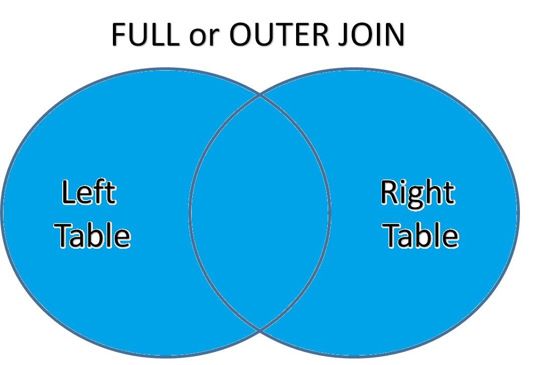
In pandas, an outer join is a method for combining two DataFrames based on a common column or index, including all rows from both DataFrames. Pandas provides the merge() function to perform joins, and the how parameter determines the type of join to execute. The syntax for an outer join in pandas is

result = pd.merge(left, right, 
                  how='outer', 
                  on=None, 
                  left_on=None, 
                  right_on=None, 
                  left_index=False, 
                  right_index=False, 
                  sort=False, 
                  suffixes=('_x', '_y'), 
                  copy=True, 
                  indicator=False, 
                  validate=None)

Here’s an explanation of each parameter:

• left: The DataFrame on the left side of the join.
• right: The DataFrame on the right side of the join.
• how: Specifies the type of join. For an outer join, set how to 'outer'. Other options include 'inner' (default), 'left', and 'right'.
• on: Column name or list of column names to join on. If None, and left_index and right_index are False, the join will be based on the intersection of the columns in both DataFrames.
• left_on: Column name or list of column names from the left DataFrame to join on.
• right_on: Column name or list of column names from the right DataFrame to join on.
• left_index: If True, use the index from the left DataFrame as the join key(s).
• right_index: If True, use the index from the right DataFrame as the join key(s).
• sort: Sort the result DataFrame by the join keys. Defaults to False.
• suffixes: Tuple of string suffixes to apply to overlapping column names from the left and right DataFrames, respectively.
• copy: If True, always copy data.
• indicator: If True, adds a special column _merge to the result DataFrame indicating the source of each row.
• validate: Checks if merge is a valid operation. Values can be 'one_to_one', 'one_to_many', 'many_to_one', or 'many_to_many'

Example

# Outer Join
​
pd.merge(left = capitals, right = currency, how = 'outer')

Notice that there is a total of 15 rows in the output above, whereas both the tables have 10 rows each. What happened here is, 5 rows are common(which came as an output of inner join) that appeared once, and the rest 5 rows of each table also got included in the final table. The values, which were not there in the tables, are filled with NaN, which is python’s way of writing Null values.

Here also, we can do the join on different column names from the left and right table, and remove the duplicates, as we saw for the inner join.

# filtering the column by using regular expressions
​
pd.merge(left = capitals,
         right = currency,
        how= 'outer',
        left_on='ISO',
        right_on='Digraph',
        suffixes=('', '_drop')).filter(regex='^(?!.*_drop)')

But here the “Country” column has Nan values for the rows not there in the left table. Hence, for outer join, it’s better to change the column name of the common value columns in such a way that both tables have the same column names and then do the outer join as seen above.

Left Join

 The left join, as demonstrated in Pandas, is a method of merging two dataframes where all rows from the left dataframe are retained, and matching rows from the right dataframe are included. Any rows from the left dataframe that do not have corresponding matches in the right dataframe will have NaN values in the columns from the right dataframe.

Here’s an example of performing a left join in Pandas:

# Left Join
left_join_result = pd.merge(left=left_dataframe, right=right_dataframe, how='left')

In this code snippet:

• left_dataframe represents the left dataframe to be merged.
• right_dataframe represents the right dataframe to be merged.
• how='left' specifies that a left join should be performed.

The resulting left_join_result dataframe will contain all rows from the left_dataframe, and matching rows from the right_dataframe. If there are no matches for a row from the left_dataframe, the corresponding columns from the right_dataframe will contain NaN values.

Left joins are particularly useful when you want to retain all records from the primary dataframe while optionally incorporating additional information from a secondary dataframe based on matching keys.

Example

# Left Join
​
pd.merge(left = capitals, right = currency, how = 'left')

Notice that there is a total of 10 rows in the output above, whereas both the tables have 10 rows each. What happened here is, only the 10 rows of the LEFT table got included in the final table. The values, which were not there in the LEFT table(Currency and Digraph), are filled with NaN, which is python’s way of writing Null values.

Note: If you have ever used Microsoft Excel or any other similar spreadsheet program, you would have done this kind of joining of data in the excel workbook. The Left Join is similar to “VLOOKUP”.

Right Join

The Right Join operation in pandas allows us to merge two dataframes, ensuring that all rows from the right dataframe are included in the final result, with matching rows from the left dataframe appended where available. Here’s how you can perform a Right Join using the merge() function in pandas:

# Performing Right Join

import pandas as pd

right_join_result = pd.merge(left=df_left, right=df_right, how='right')

print(right_join_result)

In this code:

• df_left represents the left dataframe.
• df_right represents the right dataframe.
• We use the pd.merge() function to perform the Right Join.
• The how parameter is set to 'right', indicating a Right Join operation.
• The result is stored in the variable right_join_result.
• Finally, we print or further manipulate right_join_result to analyze the joined data.

This operation ensures that all rows from the right dataframe are included, with corresponding rows from the left dataframe added where matches are found. Any non-matching rows from the left dataframe will contain NaN values in the merged dataframe.

Example

# Right Join
​
pd.merge(left = capitals, right = currency, how = 'right')

Notice that there is a total of 10 rows in the output above, whereas both the tables have 10 rows each. What happened here is, only the 10 rows of the RIGHT table got included in the final table. The values, which were not there in the RIGHT table(ISO and Capital), are filled with NaN, which is python’s way of writing Null values.

Removing the Duplicate Columns after JOIN

One apparent issue which crept into the result is duplication of the “Country” column, and you may notice that the column names have now suffix that is provided as default. There is no way in the function parameters to avoid this duplication, but a clean and smart workaround may be used in the same line of code. We can smartly use the suffixes= for this purpose.

I am going to add “_drop” suffix to the duplicate column.

Example

# filtering the column by using regular expressions
​
pd.merge(left = capitals,
         right = currency,
        how= 'inner',
        left_on='ISO',
        right_on='Digraph',
        suffixes=('', '_drop')).filter(regex='^(?!.*_drop)')

Output:

Conclusion

In conclusion, the ability to join dataframes efficiently is a fundamental aspect of data science and manipulation, especially when working with structured data in Python. Pandas provides powerful tools for merging and joining dataframes, mirroring the functionality of SQL joins.

Throughout this tutorial, we’ve explored various types of joins, such as inner join, outer join, left outer join, and right outer join, demonstrating how to perform these operations using the merge() function in Pandas. Understanding these join operations is essential for querying and extracting meaningful insights from relational databases, enabling analysts and data scientists to work effectively with large datasets and derive valuable conclusions. By mastering the concepts and techniques presented here, Python users can elevate their data analysis skills and tackle complex data integration tasks for machine learning and data analysis with confidence.

Apart from Joins, many other popular SQL functions are easily implementable in Python. Read “15 Pandas functions to replicate basic SQL Queries in Python” for learning how to do that.

The implied learning in this article was, that you can use Python to do things that you thought were only possible using SQL. There may or may not be straight forward solution to things, but if you are inclined to find it, there are enough resources at your disposal to find a way out.

Frequently Asked Questions

Nilabh Nishchhal 23 Feb 2024