What is LSTM for Text Classification?
With an emerging field of deep learning, performing complex operations has become faster and easier. As you start exploring the field of deep learning, you are definitely going to come across words like Neural networks, recurrent neural networks, LSTM, GRU, etc. This article explains LSTM Python and its use in Text Classification.
Table of contents
This article was published as a part of the Data Science Blogathon.
What is LSTM?
LSTM stands for Long-Short Term Memory. LSTM is a type of recurrent neural network but is better than traditional recurrent neural networks in terms of memory. Having a good hold over memorizing certain patterns LSTMs perform fairly better. As with every other NN, LSTM can have multiple hidden layers and as it passes through every layer, the relevant information is kept and all the irrelevant information gets discarded in every single cell. How does it do the keeping and discarding you ask?
Why LSTM?
Tradition neural networks suffer from short-term memory. Also, a big drawback is the vanishing gradient problem. ( While backpropagation the gradient becomes so small that it tends to 0 and such a neuron is of no use in further processing.) LSTMs efficiently improves performance by memorizing the relevant information that is important and finds the pattern.
How does LSTM Work in Python?
LSTM has 3 main gates:
- FORGET Gate
- INPUT Gate
- OUTPUT Gate
Let’s have a quick look at them one by one.
FORGET Gate
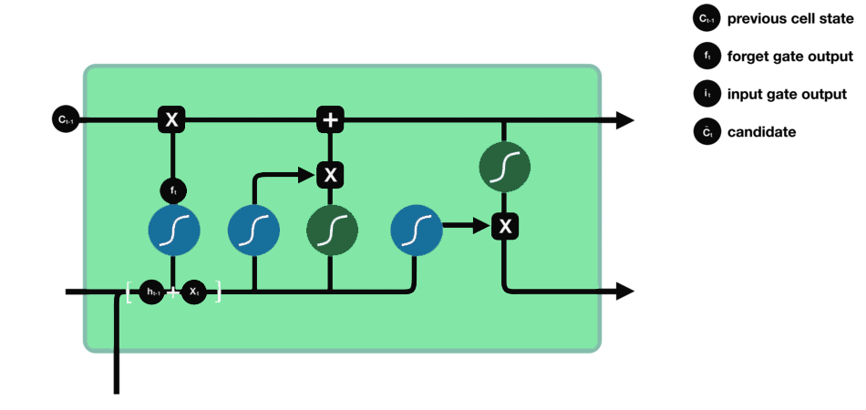
This gate is responsible for deciding which information is kept for calculating the cell state and which is not relevant and can be discarded. The ht-1 is the information from the previous hidden state (previous cell) and xt is the information from the current cell. These are the 2 inputs given to the Forget gate. They are passed through a sigmoid function and the ones tending towards 0 are discarded, and others are passed further to calculate the cell state.

INPUT Gate
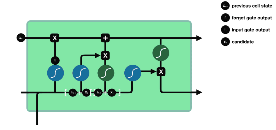
Input Gate updates the cell state and decides which information is important and which is not. As forget gate helps to discard the information, the input gate helps to find out important information and store certain data in the memory that relevant. ht-1 and xt are the inputs that are both passed through sigmoid and tanh functions respectively. tanh function regulates the network and reduces bias.

Cell State
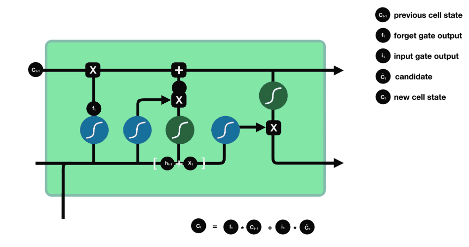
All the information gained is then used to calculate the new cell state. The cell state is first multiplied with the output of the forget gate. This has a possibility of dropping values in the cell state if it gets multiplied by values near 0. Then a pointwise addition with the output from the input gate updates the cell state to new values that the neural network finds relevant.

OUTPUT Gate
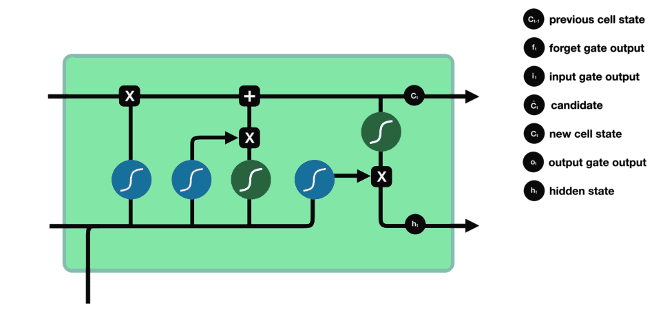
The last gate which is the Output gate decides what the next hidden state should be. ht-1 and xt are passed to a sigmoid function. Then the newly modified cell state is passed through the tanh function and is multiplied with the sigmoid output to decide what information the hidden state should carry.

LSTM Python for Text Classification
There are many classic classification algorithms like Decision trees, RFR, SVM, that can fairly do a good job, then why to use LSTM for classification?
One good reason to use LSTM is that it is effective in memorizing important information.
If we look and other non-neural network classification techniques they are trained on multiple word as separate inputs that are just word having no actual meaning as a sentence, and while predicting the class it will give the output according to statistics and not according to meaning. That means, every single word is classified into one of the categories.
This is not the same in LSTM. In LSTM we can use a multiple word string to find out the class to which it belongs. This is very helpful while working with Natural language processing. If we use appropriate layers of embedding and encoding in LSTM, the model will be able to find out the actual meaning in input string and will give the most accurate output class. The following code will elaborate the idea on how text classification is done using LSTM.
Model Defining
Defining the LSTM python model to train the data on.
Code
#model


embedding_vector_features=45

model=Sequential()

model.add(Embedding(voc_size,embedding_vector_features,input_length=sent_length))

model.add(LSTM(128,input_shape=(embedded_docs.shape),activation='relu',return_sequences=True))

model.add(Dropout(0.2))

model.add(LSTM(128,activation='relu'))

model.add(Dropout(0.2))

# for units in [128,128,64,32]:

# model.add(Dense(units,activation='relu'))

# model.add(Dropout(0.2))

model.add(Dense(32,activation='relu'))

model.add(Dropout(0.2))

model.add(Dense(4,activation='softmax'))

model.compile(loss='sparse_categorical_crossentropy',optimizer='adam',metrics=['accuracy'])

print(model.summary())
Summary
Model: "sequential_2"

_________________________________________________________________

Layer (type) Output Shape Param #
=================================================================

embedding_2 (Embedding) (None, 35, 45) 360000
_________________________________________________________________

lstm_4 (LSTM) (None, 35, 128) 89088
_________________________________________________________________

dropout_6 (Dropout) (None, 35, 128) 0
_________________________________________________________________

lstm_5 (LSTM) (None, 128) 131584
_________________________________________________________________

dropout_7 (Dropout) (None, 128) 0
_________________________________________________________________

dense_4 (Dense) (None, 32) 4128
_________________________________________________________________

dropout_8 (Dropout) (None, 32) 0
_________________________________________________________________

dense_5 (Dense) (None, 4) 132
=================================================================

Total params: 584,932
Trainable params: 584,932
Non-trainable params: 0
_________________________________________________________________
We define a sequential model and add various layers to it.
Explanation
The first layer is Embedding layer. It representing words using a dense vector representation. The position of a word within the vector space is based on the words that surround the word when it is used. For eg. “king” is placed near “man” and “queen” is placed near “woman”. The vocabulary size is provided.
The next layer is an LSTM layer with 128 neurons. “embedded_docs” is the input list of sentences which is one hot encoded and every sentence is made of the same length. The activation function is rectified linear, which widely used. Any other relevant activation function can be used. “return_sequences=True” this is an important parameter while using multiple LSTM layer as it enables the output of the previous LSTM layer to be used as an input to the next LSTM layer. If it is not set to true, the next LSTM layer will not get the input.
A dropout layer is used for regulating the network and keeping it as away as possible from any bias. Another LSTM layer with 128 cells followed by some dense layers.
The final Dense layer is the output layer which has 4 cells representing the 4 different categories in this case. The number can be changed according to the number of categories.
Compiling the model using adam optimizer and sparse_categorical_crossentropy. Adam optimizer is the current best optimizer for handling sparse gradients and noisy problems. The sparse_categorical_crossentropy is mostly used when the classes are mutually exclusive, ie, when each sample belongs to exactly one class. The Summary explains all the details of the model.
Training the Model for LSTM Python
Now that the model is ready, the data to be trained it split into train data and test data. Here the split is 90-10. X_final and y_final are the independent and dependent datasets.
Code:
from sklearn.model_selection import train_test_split
X_train, X_test, y_train, y_test = train_test_split(X_final, y_final, test_size=0.1, random_state=42,stratify=y_final)
The next step is to train the LSTM model using the train data, and the test data is used for validating. Model.fit() is used for this purpose.
Code:
model.fit(X_train,y_train,validation_data=(X_test,y_test),epochs=120,batch_size=64)The epochs are the number of times the process will be repeated. It can be 20,120, 2000, 20000, any number. The batch size is 64, ie, for every epoch, a batch of 64 inputs will be used to train the model. It mostly depends on how large the dataset is.
Prediction
After training is completed, it’s time to find out the result and predict using the model.
Accuracy
Code:
results = model.evaluate(X_test,y_test)The model is evaluated and the accuracy of how well the model classifies the data is calculated. “results” will have the accuracy score and the loss. In some cases increasing the number of epochs can increase the accuracy as the model gets trained better.
To use the trained model for predicting, the predict() function is used.
Predict
Code:
The “embedded_docs_pred” is the list is words or sentences that is to be classified and is one-hot encoded and padded to make them of equal length.
y_pred = model.predict(embedded_docs_pred)
y_pred:

array([[2.65598774e-01, 2.36345261e-01, 4.28116888e-01, 6.99390173e-02],
       [2.47113910e-02, 9.56604779e-01, 3.82159604e-03, 1.48621844e-02],
       [1.53286534e-03, 9.94825006e-01, 1.15779374e-04, 3.52645456e-03],
       [5.94987810e-01, 3.00740451e-01, 7.62206316e-02, 2.80511230e-02]])
The output will have a list for every input (can be a word or a sentence). Every list has the predicted score for 4 classes. The maximum of them is the class for that respective input. As discussed above LSTM facilitated us to give a sentence as an input for prediction rather than just one word, which is much more convenient in NLP and makes it more efficient.
Conclusion
In conclusion, LSTM (Long Short-Term Memory) models have proven to be a powerful tool for text classification in Python. With their ability to capture long-term dependencies and handle sequential data, LSTM models offer improved accuracy in classifying text. By implementing LSTM models in Python, researchers and practitioners can leverage the strengths of this architecture to achieve better results in various text classification tasks, opening up new possibilities for natural language processing applications. Sign-up for our Blackbelt program if you want to learn more about it!
Frequently Asked Questions
A. Yes, LSTM (Long Short-Term Memory) networks are commonly used for text classification tasks due to their ability to capture long-range dependencies in sequential data like text.
A. Yes, LSTM can indeed be employed for text generation tasks. Its ability to learn patterns and generate sequences makes it suitable for applications like generating text in various domains.
A. Absolutely, LSTM is widely used in natural language processing (NLP) tasks such as sentiment analysis, machine translation, and named entity recognition due to its effectiveness in handling sequential data like language.
A. Yes, LSTM can be effective for classification tasks in NLP due to its ability to capture intricate patterns and dependencies in text data, leading to accurate predictions in tasks such as sentiment analysis or document classification.
The media shown in this article on LSTM for Text Classification are not owned by Analytics Vidhya and are used at the Author’s discretion.


Hi Shraddha, Thank you for this great blog. I got an error when I reshape the input for the LSTM, can you advise me why i got this error and how to solve it. When I reshape the trainingg and testing set: # Reshape the input to shape (num_instances, timesteps, num_features) train_data = train_data.reshape(train_data.shape[0], 1, train_data.shape[1]) test_data=test_data.reshape(test_data.shape[0],1,test_data.shape[1]) #Fit the model history = model.fit(train_data, train_labels, epochs=epochs, batch_size=batch_size, validation_data=(test_data, test_labels), callbacks=[callback]) I got this error : ValueError: Shapes (None,) and (None, 1, 5) are incompatible Thank you in Advance