This article was published as a part of the Data Science Blogathon
This article is part of an ongoing blog series on Natural Language Processing (NLP). Up to the previous part of this article series, we almost completed the necessary steps involved in text cleaning and normalization pre-processing. After that, we will convert the processed text to numeric feature vectors so that we can feed it to computers for Machine Learning applications.
NOTE: Some concepts included in the pipeline of text preprocessing aren’t discussed yet such as Parsing, Grammar, Named Entity Recognition, etc which we will cover after complete the concepts of word embedding so that you can try to make a small project on NLP by using all the concepts covered till now in this series and increase your understanding of all the concepts.
So, In this article, we will understand the Word Embeddings with their types and discuss all the techniques covered in each of the types of word embeddings. Nowadays more recent Word Embedding approaches are used to carry out most of the downstream NLP tasks. So, In this article lets us look at pre word embedding era of text vectorization approaches.
This is part-5 of the blog series on the Step by Step Guide to Natural Language Processing.
1. Familiar with Terminologies
2. What is Word Embedding?
3. Different Types of Word Embeddings
4. Pre word embedding era Techniques
Before understanding Vectorization, below are the few terms that you need to understand.
A document is a single text data point. For Example, a review of a particular product by the user.
It a collection of all the documents present in our dataset.
Every unique word in the corpus is considered as a feature.
For Example, Let’s consider the 2 documents shown below:
Sentences:
Dog hates a cat. It loves to go out and play.
Cat loves to play with a ball.
We can build a corpus from the above 2 documents just by combining them.
Corpus = “Dog hates a cat. It loves to go out and play. Cat loves to play with a ball.”
And features will be all unique words:
Fetaures: [‘and’, ‘ball’, ‘cat’, ‘dog’, ‘go’, ‘hates’, ‘it’, ‘loves’, ‘out’, ‘play’, ‘to’, ‘with’]
We will call it a feature vector. Here we remember that we will remove ‘a’ by considering it a single character.
In very simple terms, Word Embeddings are the texts converted into numbers and there may be different numerical representations of the same text. But before we dive into the details of Word Embeddings, the following question should come to mind:
As we know that many Machine Learning algorithms and almost all Deep Learning Architectures are not capable of processing strings or plain text in their raw form. In a broad sense, they require numerical numbers as inputs to perform any sort of task, such as classification, regression, clustering, etc. Also, from the huge amount of data that is present in the text format, it is imperative to extract some knowledge out of it and build any useful applications.
In short, we can say that to build any model in machine learning or deep learning, the final level data has to be in numerical form because models don’t understand text or image data directly as humans do.
So, another question that may also come to mind is given:
To convert the text data into numerical data, we need some smart ways which are known as vectorization, or in the NLP world, it is known as Word embeddings.
Therefore, Vectorization or word embedding is the process of converting text data to numerical vectors. Later those vectors are used to build various machine learning models. In this manner, we say this as extracting features with the help of text with an aim to build multiple natural languages, processing models, etc. We have different ways to convert the text data to numerical vectors which we will discuss in this article later.
Let’s now define the Word Embeddings formally,
A Word Embedding generally tries to map a word using a dictionary to its vector form.
Do you think that Word Embedding and Text Vectorization are the same things or there is no difference at all between these two techniques? If yes, Why and If No, then what is the exact difference between these two techniques?
Broadly, we can classified word embeddings into the following two categories:
In this technique, we represent each unique word in vocabulary by setting a unique token with value 1 and rest 0 at other positions in the vector. In simple words, a vector representation of a one-hot encoded vector represents in the form of 1, and 0 where 1 stands for the position where the word exists and 0 everywhere else.
Image Source: Google Images
Let’s consider the following sentence:
Sentence: I am teaching NLP in Python
A word in this sentence may be “NLP”, “Python”, “teaching”, etc.
Since a dictionary is defined as the list of all unique words present in the sentence. So, a dictionary may look like –
Dictionary: [‘I’, ’am’, ’teaching’,’ NLP’,’ in’, ’Python’]
Therefore, the vector representation in this format according to the above dictionary is
Vector for NLP: [0,0,0,1,0,0]
Vector for Python:  [0,0,0,0,0,1]
This is just a very simple method to represent a word in vector form.
1. One of the disadvantages of One-hot encoding is that the Size of the vector is equal to the count of unique words in the vocabulary.
2. One-hot encoding does not capture the relationships between different words. Therefore, it does not convey information about the context.
1. It is one of the simplest ways of doing text vectorization.
2. It creates a document term matrix, which is a set of dummy variables that indicates if a particular word appears in the document.
3. Count vectorizer will fit and learn the word vocabulary and try to create a document term matrix in which the individual cells denote the frequency of that word in a particular document, which is also known as term frequency, and the columns are dedicated to each word in the corpus.

Image Source: Google Images
Consider a Corpus C containing D documents {d1,d2…..dD} from which we extract N unique tokens. Now, the dictionary consists of these N tokens, and the size of the Count Vector matrix M formed is given by D X N. Each row in the matrix M describes the frequency of tokens present in the document D(i).
Let’s consider the following example:
Document-1: He is a smart boy. She is also smart.
Document-2: Chirag is a smart person.
The dictionary created contains the list of unique tokens(words) present in the corpus
Unique Words: [‘He’, ’She’, ’smart’, ’boy’, ’Chirag’, ’person’]
Here, D=2, N=6
So, the count matrix M of size 2 X 6 will be represented as –
| He | She | smart | boy | Chirag | person | |
| D1 | 1 | 1 | 2 | 1 | 0 | 0 |
| D2 | 0 | 0 | 1 | 0 | 1 | 1 |
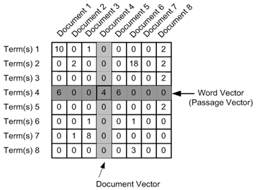
Now, a column can also be understood as a word vector for the corresponding word in the matrix M.
For Example, for the above matrix formed, let’s see the word vectors generated.
Vector for ‘smart’ is [2,1],
Vector for ‘Chirag’ is [0, 1], and so on.
Another way to read the D2 or the second row in the above matrix is shown below:
‘lazy’: once, ‘Neeraj’: once, and ‘person’ once
Now, Let’s discuss some of the variations while preparing the above matrix M. The variations will be generally in the following ways:
Since the matrix, we prepared above is the sparse matrix, which is inefficient for any computations. So, to deal with this problem we can make this variation. The idea behind this variation is that in real-world applications we might have a corpus that has millions of documents and with the help of these millions of documents, we can extract hundreds of millions of unique words which is a very huge number. So, now as an alternative, we prepare our dictionary using every unique word as a dictionary element and we would pick say only the top 5000 words based on the frequency.
We have the following two options in hand for entry in the count matrix-
But in general, we preferred the frequency method over the latter.
Below represents an image of the matrix M for easy understanding.
Image Source: Google Images
This vectorization technique converts the text content to numerical feature vectors. Bag of Words takes a document from a corpus and converts it into a numeric vector by mapping each document word to a feature vector for the machine learning model.
Image Source: Google Images
In this approach of text vectorization, we perform two operations.
It is the process of dividing each sentence into words or smaller parts, which are known as tokens. After the completion of tokenization, we will extract all the unique words from the corpus. Here corpus represents the tokens we get from all the documents and used for the bag of words creation.
Here the vector size for a particular document is equal to the number of unique words present in the corpus. For each document, we will fill each entry of a vector with the corresponding word frequency in a particular document.
Let’s take a good understanding with the help of the following example:
This burger is very tasty and affordable
This burger is not tasty and is affordable
This burger is very very delicious
These 3 sentences are example sentences and combined it forms a corpus and our first step is to perform tokenization. Before tokenization, we will convert all sentences to lowercase letters or uppercase letters. Here, for normalization, we will convert all the words in the sentences to lowercase.
Now, the Output of sentences after converting to lowercase is:
this burger is very tasty and affordable.
this burger is not tasty and is affordable.
this burger is very very delicious.
Now we will perform tokenization.
After dividing the sentences into words and generate a list with all unique words in alphabetical order, we will get the following output after the tokenization step:
Unique words: [“and”, “affordable.”, “delicious.”, “is”, “not”, “burger”, “tasty”, “this”, “very”]
Now, what is our next step?
Creating vectors for each sentence with the frequency of words. This is called a sparse matrix. Below is the sparse matrix of example sentences.
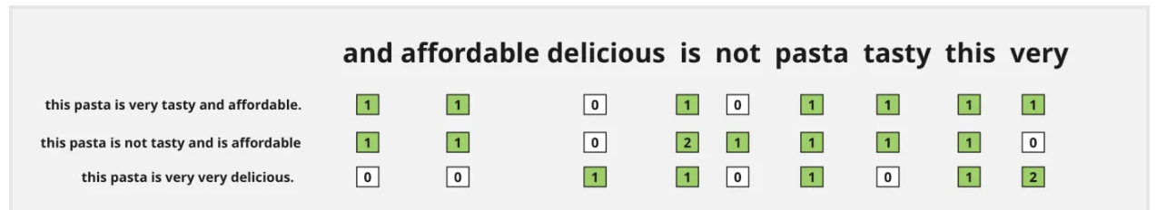
Therefore, as we discussed here each document is represented as an array having a size same as the length of the total numbers of features. All the values of this array will be zero apart from one position and that position representing words address inside the feature vector.
The final BoW representation is the sum of the words feature vector.
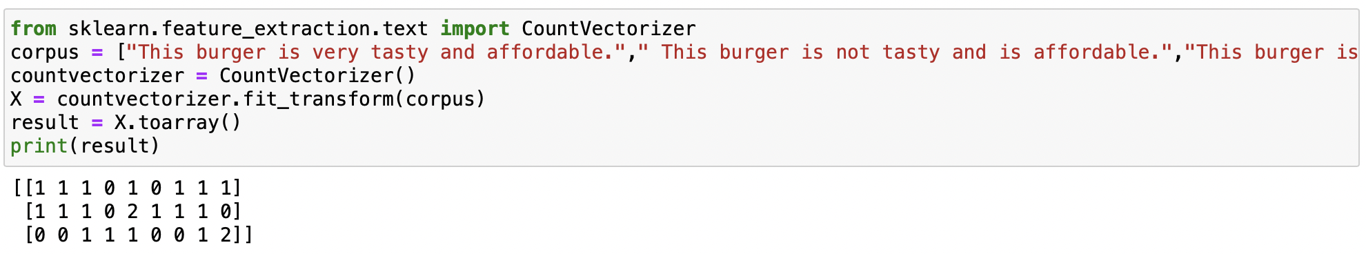
Now, the implementation of the above example in Python is given below:
1. This method doesn’t preserve the word order.
2. It does not allow to draw of useful inferences for downstream NLP tasks.
Do you think there is some kind of relationship between the two techniques which we completed – Count Vectorizer and Bag of Words? Why or Why not?
1. Similar to the count vectorization technique, in the N-Gram method, a document term matrix is generated, and each cell represents the count.
2. The columns represent all columns of adjacent words of length n.
3. Count vectorization is a special case of N-Gram where n=1.
4. N-grams consider the sequence of n words in the text; where n is (1,2,3.. ) like 1-gram, 2-gram. for token pair. Unlike BOW, it maintains word order.
For Example,
“I am studying NLP” has four words and n=4.
if n=2, i.e bigram, then the columns would be — [“I am”, “am reading”, ‘studying NLP”]
if n=3, i.e trigram, then the columns would be — [“I am studying”, ”am studying NLP”]
if n=4,i.e four-gram, then the column would be -[‘“I am studying NLP”]
The n value is chosen based on the performance.
The trade-off is created while choosing the N values. If we choose N as a smaller number, then it may not be sufficient enough to provide the most useful information. But on the contrary, if we choose N as a high value, then it will yield a huge matrix with lots of features. Therefore, N-gram may be a powerful technique, but it needs a little more care.
1. It has too many features.
2. Due to too many features, the feature set becomes too sparse and is computationally expensive.
3. Choose the optimal value of N is not that easy task.
As we discussed in the above techniques that the BOW method is simple and works well, but the problem with that is that it treats all words equally. As a result, it cannot distinguish very common words or rare words. So, to solve this problem, TF-IDF comes into the picture!
Term frequency-inverse document frequency ( TF-IDF) gives a measure that takes the importance of a word into consideration depending on how frequently it occurs in a document and a corpus.
To understand TF-IDF, firstly we will understand the two terms separately:
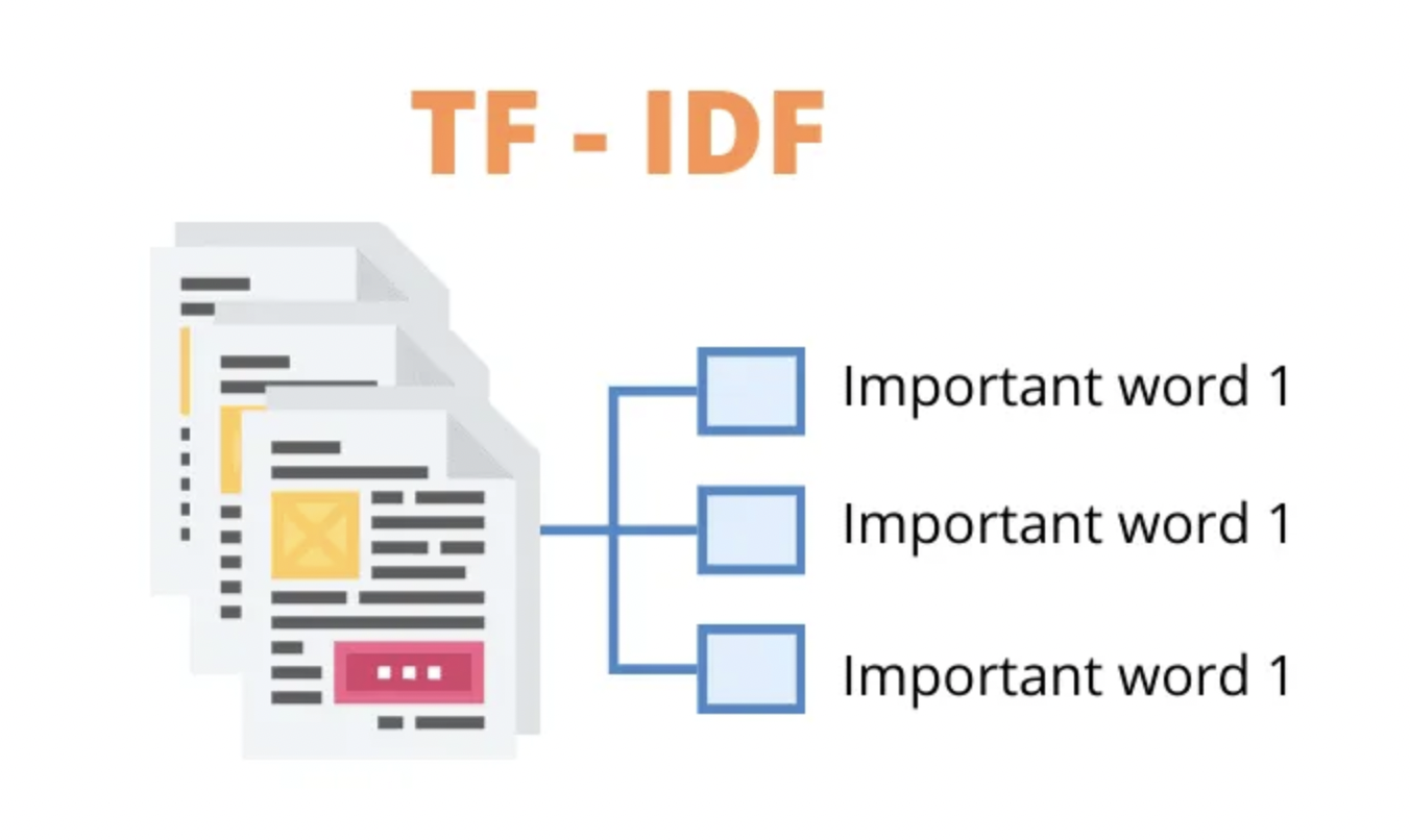
Image Source: Google Images
Term frequency denotes the frequency of a word in a document. For a specified word, it is defined as the ratio of the number of times a word appears in a document to the total number of words in the document.
Or, it is also defined in the following manner:
It is the percentage of the number of times a word (x) occurs in a particular document (y) divided by the total number of words in that document.
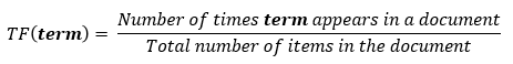
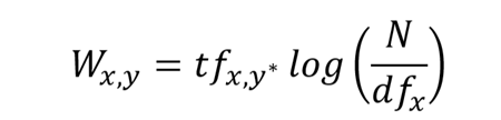
The formula for finding Term Frequency is given as:
tf (‘word’) = Frequency of a ‘word’ appears in document d / total number of words in the document d
For Example, Consider the following document
Document: Cat loves to play with a ball
For the above sentence, the term frequency value for word cat will be: tf(‘cat’) = 1 / 6
Note: Sentence “Cat loves to play with a ball” has 7 total words but the word ‘a’ has been ignored.
It measures the importance of the word in the corpus. It measures how common a particular word is across all the documents in the corpus.
It is the logarithmic ratio of no. of total documents to no. of a document with a particular word.
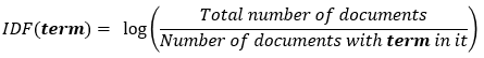
This term of the equation helps in pulling out the rare words since the value of the product is maximum when both the terms are maximum. What does that mean? If a word appears multiple times across many documents, then the denominator df will increase, reducing the value of the second term. (Refer to the formula given below)
The formula for finding Inverse Document Frequency is given as:
idf(‘word’) = log(Total number of documents / number of document with ‘word’ in it)
Here the main idea is to find the common or rare words.
For Example, In any corpus, few words like ‘is’ or ‘and’ are very common, and most likely, they will be present in almost every document.
Let’s say the word ‘is’ is present in all the documents is a corpus of 1000 documents. The idf for that would be:
The idf(‘is’) is equal to log (1000/1000) = log 1 = 0
Thus common words would have lesser importance.
![]()
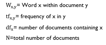
The formula for finding TF-IDF is given as:
where,
In the same way, the idf(‘cat’) will be equal to 0 in our example.
The tf-idf is equal to the product of tf and idf values for that word:
Therefore, tf-idf(‘cat’ for document 2) = tf(‘cat’) * idf(‘cat’) = 1 / 6 * 0 = 0
Thus, tf-idf(‘cat’) for document 2 would be 0
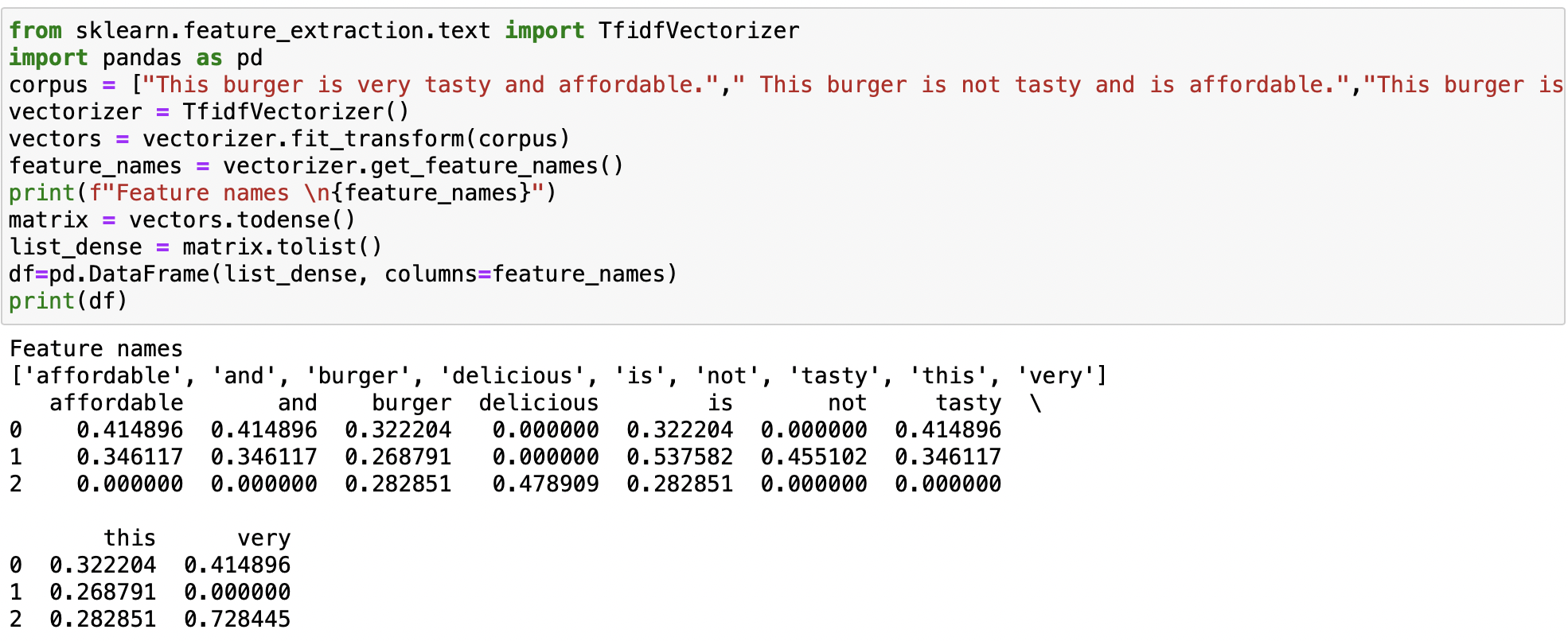
1. Similar to the count vectorization method, in the TF-IDF method, a document term matrix is generated and each column represents an individual unique word.
2. The difference in the TF-IDF method is that each cell doesn’t indicate the term frequency, but contains a weight value that signifies how important a word is for an individual text message or document
3. This method is based on the frequency method but it is different from the count vectorization in the sense that it takes into considerations not just the occurrence of a word in a single document but in the entire corpus.
4. TF-IDF gives more weight to less frequently occurring events and less weight to expected events. So, it penalizes frequently occurring words that appear frequently in a document such as “the”, “is” but assigns greater weight to less frequent or rare words.
5. The product of TF x IDF of a word indicates how often the token is found in the document and how unique the token is to the whole entire corpus of documents.
Now, the implementation of the example discussed in BOW in Python is given below:
Do you think there can be some variations of the TF-IDF technique based on some criteria? If yes, then mention those variations, and if no, then why?
All of these techniques we discussed here suffer from the issue of vector sparsity and as a result, it doesn’t handle complex word relations and is not able to model long sequences of text. So, In the next part of this series, we’ll try to look at new-age text vectorization techniques, that tries to overcome this problem.
You can also check my previous blog posts.
Previous Data Science Blog posts.
Here is my Linkedin profile in case you want to connect with me. I’ll be happy to be connected with you.
For any queries, you can mail me on Gmail.
Thanks for reading!
I hope that you have enjoyed the article. If you like it, share it with your friends also. Something not mentioned or want to share your thoughts? Feel free to comment below And I’ll get back to you. 😉
The media shown in this article are not owned by Analytics Vidhya and are used at the Author’s discretion.
I am currently pursuing my Bachelor of Technology (B.Tech) in Computer Science and Engineering from the Indian Institute of Technology Jodhpur(IITJ). I am very enthusiastic about Machine learning, Deep Learning, and Artificial Intelligence. Feel free to connect with me on Linkedin.
Lorem ipsum dolor sit amet, consectetur adipiscing elit,