This article was published as a part of the Data Science Blogathon
Overview
In this blog, we will be exploring the basic concepts of time series along with small hands-on python implementations. The concepts explained here are expressed as simply as possible to help you further build your knowledge in time series modelling. Happy Learning!
Table of Contents
1.Introduction
2.Basic Components of a time series
3.Stationary vs Non-stationary time series data
3.Code implementation
4.Conclusion
5.Reference
Introduction
What is Time Series?
Time series is basically sequentially ordered data indexed over time. Here time is the independent variable while the dependent variable might be
- Stock market data
- Sales data of companies
- Data from the sensors of smart devices
- The measure of electrical energy generated in the powerhouse.
Well, those were some of the examples and the list may go on. To gain some useful insights from time-series data, you have to decompose the time series and look for some basic components such as trend, seasonality, cyclic behaviour, and irregular fluctuations. Based on some of these behaviours, we are deciding on which model to choose for time series modelling. These concepts will be explained to you in the upcoming part, but I will give you a small introduction about some of these terms. Assume that you are having the time-series data of an airline passenger company, if you do an initial analysis on the data, you can find that in each year during particular periods of time, a particular pattern may be found(a seasonal pattern). Further investigating we may find that it was because vacations were happening in those months because of which families were travelling. Also, you may be able to find other insights like an increase/decrease in the passenger count(upward/downward trend), which may be related to some other factors that were affecting the airlines at that time. Let’s get a better understanding of these terms by examining the time series plots themselves.
Basic Components of Time series
Seasonality
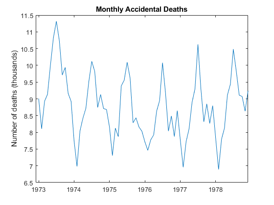
Source: https://ww2.mathworks.cn/help/econ/seasonal-adjustment.html
This data contains the record of the total number of deaths happening in a month. If we are taking a fixed time span of one year, we can find that by mid of each year there is a surge in the number of deaths occurring. This pattern is visible every year that we have observed. So, this is basically the seasonality present in the data. So if we say that a time series has seasonality, it implies that there are repeating patterns of almost constant length occurring over time. Keep in mind that the time series model which takes into account seasonality is SARIMA.
Trend
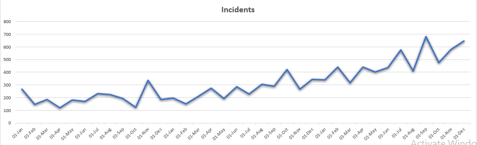
Source: https://www.aptech.com/blog/introduction-to-the-fundamentals-of-time-series-data-and-analysis/
Analyzing this series we can observe that as we move along the horizontal axis, the value in the vertical axis is increasing. This is basically the trend i.e the linear increment or a decrement in the observed value as the recorded series progress over time. When it comes to time series modelling we usually remove these trends that are present in the series.
Cyclic behaviour

Source : Furthermaths(https://www.youtube.com/watch?v=ca0rDWo7IpI&t=529s)
Don’t confuse cyclic behaviour with seasonality because, in seasonality, a predictable pattern is observed in a regular interval of time, while in a cyclic variation the peaks and troughs don’t occur in a regular interval of time. From the above image, we can see that the peaks are occurring at different times, the time gap is not regular. People always get confused about seasonality and cyclic behaviour. Wrong inferencing may affect your result while choosing the model for time series forecasting.
Combining everything in a single picture,
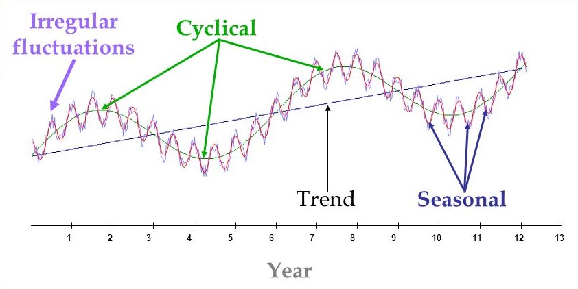
Source: https://github.com/ashishpatel26/ML-Notes-in-Markdown/blob/master/11-TimeSeries/01-Introduction.md
So that’s the theory. Now let us try some python code to decompose a given time series to the respective components
Stationary vs Non-Stationary data
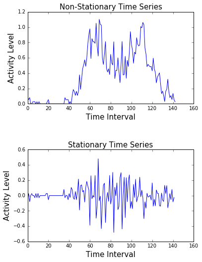
Source: https://www.researchgate.net/publication/326619835_Call_Detail_Records_Driven_Anomaly_Detection_and_Traffic_Prediction_in_Mobile_Cellular_Networks
Well, this is not actually a component of time series data, but these are the types of time series data that you may observe in the real world. If you keenly observe the above images you can find the difference between the two plots. In stationary time series the mean, variance, and standard deviation of the observed value over time are almost constant whereas in non-stationary time series this is not the case. So basically initially as a first step, we can check whether the time series is stationary or not, and if it’s not stationary we can apply some transformations to make it so. It is important to make time-series data stationary because a lot of statistical analysis and modelling depend upon stationary data. To check stationarity, we can perform tests such as the ADF (Augmented Dickey-Fuller) test which provides us a better intuition.
Code Implementation
Here we are going to take the dataset containing a monthly count of riders for the Portland transportation system.
1.Importing Necessary libraries
import pandas as pd
import matplotlib.pyplot as plt
2.Loading the data as a data frame
df=pd.read_csv('https://raw.githubusercontent.com/josephofiowa/GA-DSI/master/example-lessons/Intro-to-forecasting/portland-oregon-average-monthly-.csv',parse_dates = ['Month'])
df.rename(columns = {'Portland Oregon average monthly bus ridership (/100) January 1973 through June 1982, n=114':'monthly_ridership'},inplace = True)
df.dropna(inplace = True)

df = df.iloc[:114]

df = df.set_index('Month')

df = df['monthly_ridership'].apply(lambda x: int(x))

rid_df = pd.DataFrame(df)
Keep in mind that you have to specifically mention the column that you wish to parse as dates while reading the CSV data.
3.An initial analysis of the time-series data
rid_df['monthly_ridership'].plot()
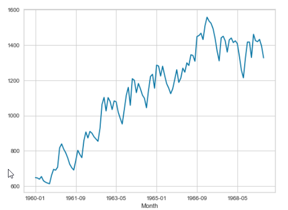
Source: https://github.com/radathan1/A-Beginners-Guide-to-Time-Series-Analysis/blob/main/A%20Beginners%20Guide%20to%20time%20series%20Analysis.ipynb
Just by observation, we can find here that the time- series has trend and seasonality present. Let us further decompose the data to the respective components.
4.Decomposing the time series data
from statsmodels.tsa.seasonal import seasonal_decompose
# Decomposing Time series
decomposition = seasonal_decompose(rid_df.monthly_ridership, freq=12)
fig = plt.figure()
fig = decomposition.plot()
fig.set_size_inches(15, 8)
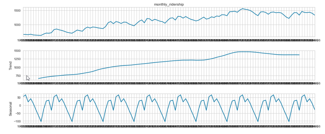
Source: https://github.com/radathan1/A-Beginners-Guide-to-Time-Series-Analysis/blob/main/A%20Beginners%20Guide%20to%20time%20series%20Analysis.ipynb
Yes, our assumptions were true there was trend and seasonality present in the data. The topmost figure is the monthly ridership data and the second and third figures show the decomposed trend and seasonality that is present respectively.
Conclusion
Here we had discussed briefly what is time series and its components. This will give a building block for you to study more on time series modelling which will include models such as ARIMA, SARIMA(Seasonal ARIMA) for forecasting the time series, which I have not explained here. Nowadays several deep-learning architectures have also been used for time series applications, these include RNN, LSTM, and Attention-based models that can remember long-term dependencies which is a crucial element in time series. I have given the link for the paper in the references, please check it out. Facebook had recently released its open-source library called Facebook Prophet for time series forecasting. It is much simpler to use for time series modelling. Finally, please try to implement the above code for decomposing the time series into its components. The entire code is available in my Github repo.
References:
1. A complete hands-on tutorial on time series analysis and Forecasting by AI_Engineer.
2. Time Series Forecasting with deep learning: A survey – Research paper.
Author
Hello, myself Adwait Dathan R currently pursuing my master’s in Artificial Intelligence and Data Science. Feel free to connect with me through LinkedIn.
Adwait Dathan R
11 Jul, 2021


