A Brief Introduction to Linear Discriminant Analysis

Introduction

Linear Discriminant Analysis (LDA), as its name suggests, serves as a linear model for classification and dimensionality reduction. You most commonly use it for feature extraction in pattern classification problems. This technique has been around for quite a long time. Initially, in 1936, Fisher formulated linear discriminant for two classes. Later on, in 1948, C.R. Rao generalized it for multiple classes. LDA projects data from a D-dimensional feature space down to a D’ (D > D’) dimensional space, thereby maximizing the variability between the classes and reducing the variability within the classes.

Learning Objectives:

• Understand the concept and purpose of Linear Discriminant Analysis (LDA)
• Learn how LDA performs dimensionality reduction and classification
• Grasp the mathematical principles behind Fisher’s Linear Discriminant
• Explore LDA implementation and applications using Python

This article was published as a part of the Data Science Blogathon

What is Linear Discriminant Analysis?

Linear Discriminant Analysis (LDA) is a statistical technique for categorizing data into groups. It identifies patterns in features to distinguish between different classes. For instance, it may analyze characteristics like size and color to classify fruits as apples or oranges. LDA aims to find a straight line or plane that best separates these groups while minimizing overlap within each class. By maximizing the separation between classes, it enables accurate classification of new data points. In simpler terms, LDA helps make sense of data by effectively finding the most efficient way to separate different categories. Consequently, this aids in tasks like pattern recognition and classification.

Why Linear Discriminant Analysis (LDA)?

• Logistic Regression is one of the most popular linear classification models that perform well for binary classification but falls short in the case of multiple classification problems with well-separated classes. While LDA handles these quite efficiently.
• Linear Discriminant Analysis (LDA) also reduces the number of features in data preprocessing, akin to Principal Component Analysis (PCA), thereby significantly reducing computing costs.
• LDA is also used in face detection algorithms. In Fisherfaces LDA is used to extract useful data from different faces. Coupled with eigenfaces it produces effective results.

Shortcomings

• Linear decision boundaries may not effectively separate non-linearly separable classes. More flexible boundaries are desired.
• In cases where the number of observations exceeds the number of features, LDA might not perform as desired. This is called Small Sample Size (SSS) problem. Regularization is required.

We will discuss this later.

Assumptions

Linear Discriminant Analysis (LDA) makes some assumptions about the data:

• It assumes that the data follows a normal or Gaussian distribution, meaning each feature forms a bell-shaped curve when plotted.
• Each of the classes has identical covariance matrices.

However, it is worth mentioning that LDA Machine Learning still performs quite well even if you violate the assumptions.

Fisher’s Linear Discriminant

Linear Discriminant Analysis in Machine Learning is a generalized form of Fisher’s Linear Discriminant (FLD). Initially, Fisher, in his paper, used a discriminant function to classify between two plant species, namely Iris Setosa and Iris Versicolor.

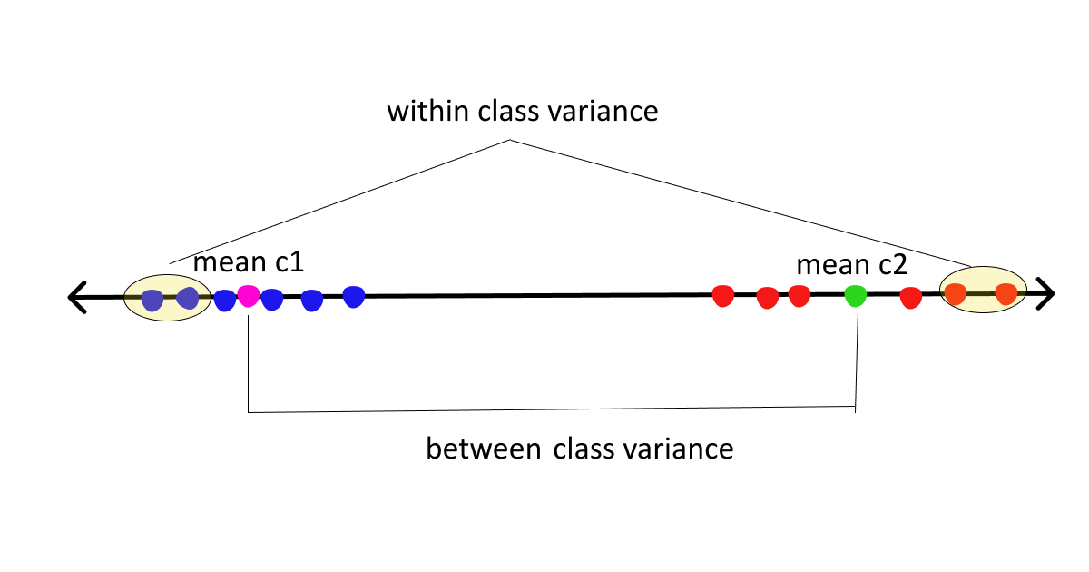
The basic idea of FLD is to project data points onto a line in order to maximize the between-class scatter and minimize the within-class scatter. Consequently, this approach aims to enhance the separation between different classes by optimizing the distribution of data points along a linear dimension.

This might sound a bit cryptic but it is quite straightforward. So, before we delve deep into the derivation part, we need to familiarize ourselves with certain terms and expressions.

• Let’s suppose we have d-dimensional data points x₁….x_n with 2 classes C_i=1,2 each having N₁ & N₂ samples.
• Consider W as a unit vector onto which we will project the data points. Since we are only concerned with the direction, we choose a unit vector for this purpose.
• Number of samples : N = N1 + N2
• If x(n) are the samples on the feature space then WTx(n) denotes the data points after projection.
• Means of classes before projection: m_i
• Means of classes after projection:  M_i = W^Tm_i

Scatter matrix: Used to make estimates of the covariance matrix. IT is a m X m positive semi-definite matrix.

Given by: sample variance * no. of samples.

Note: Scatter and variance measure the same thing but on different scales. So, we might use both words interchangeably. So, do not get confused.

Two Types of Scatter Matrices

Here we will be dealing with two types of scatter matrices

• Between class scatter = S_b = measures the distance between class means
• Within class scatter = Sw = measures the spread around means of each class

Now, assuming we are clear with the basics let’s move on to the derivation part.

As per Fisher’s LDA :

arg max J(W) = (M1 - M2)2 / S12 + S22       ...........    (1)

The numerator here is between class scatter while the denominator is within-class scatter. So to maximize the function we need to maximize the numerator and minimize the denominator, simple math. To maximize the above function we need to first express the above equation in terms of W. 

Numerator

Denominator

For denominator we have S₁² + S₂²  . 

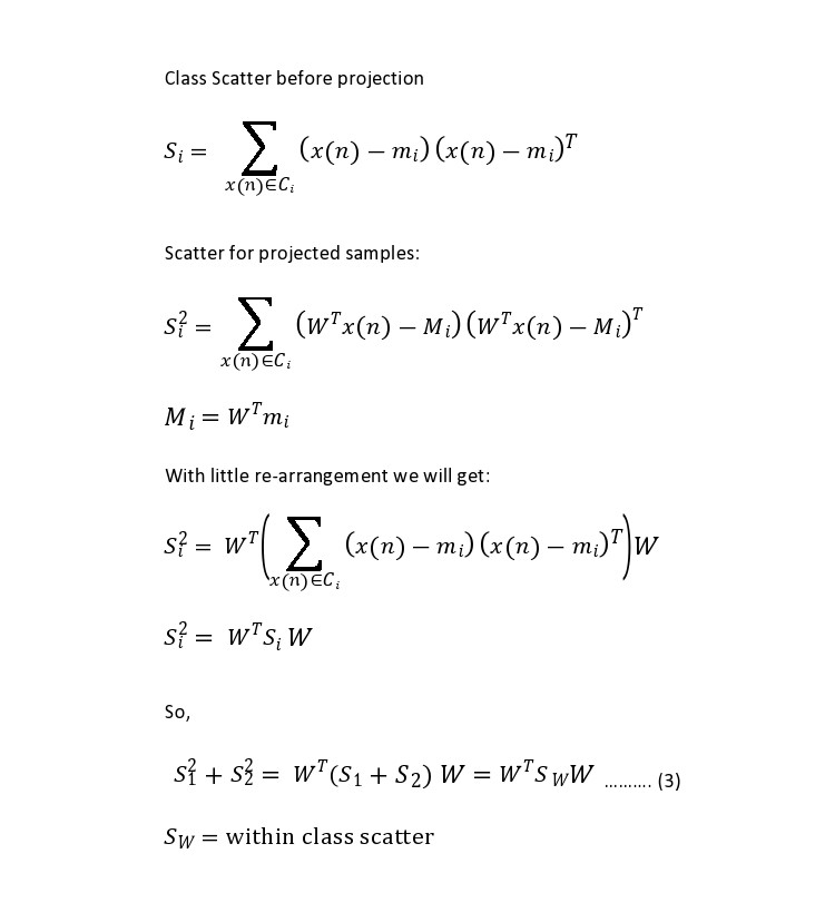
Now, we have both the numerator and denominator expressed in terms of W

J(W) = WTSbW / WTSwW

Upon differentiating the above function w.r.t W and equating with 0, we get a generalized eigenvalue-eigenvector problem

SbW = vSwW    

S_w being a full-rank matrix , inverse is feasible

=> Sw-1SbW = vW

Where v = eigen value

W = eigen vector

Linear Discriminant Analysis (LDA) for multiple classes:

Linear Discriminant Analysis (LDA) can be generalized for multiple classes. Here are the generalized forms of between-class and within-class matrices.

Note: S_b is the sum of C different rank 1 matrices. So, the rank of S_b <=C-1. That means we can only have C-1 eigenvectors. Thus, we can project data points to a subspace of dimensions at most  C-1.

Above equation (4) gives us scatter for each of our classes and equation (5) adds all of them to give within-class scatter. Similarly, equation (6) gives us between-class scatter. Finally, eigen decomposition of S_w^-1S_b gives us the desired eigenvectors from the corresponding eigenvalues. Total eigenvalues can be at most C-1.

LDA for classification:

Until now, we only reduced the dimension of the data points, but this is strictly not yet discriminant. You can subsequently use the projected data to construct a discriminant by applying Bayes’ theorem as follows.

Assume a multivariate Gaussian distribution draws X = (x1….xp). Let K represent the number of classes, and Y be the response variable. Additionally, let pik denote the prior probability, which is the probability that a given observation associates with the Kth class. Moreover, Pr(X = x | Y = k) represents the posterior probability.

Let f_k(X) = Pr(X = x | Y = k) is our probability density function of X for an observation x that belongs to K^th class. f_k(X) is large if there is a high probability of an observation in  K^th class has X=x. 

Bayes’ theorem:

Now, to calculate the posterior probability we will need to find the prior pi_k and density function f_k(X). 

pik can be calculated easily. If we have a random sample of Ys from the population: we simply compute the fraction of the training observations that belong to Kth class. But the calculation of f_k(X) can be a little tricky.

We assume that the probability density function of x is multivariate Gaussian with class means m_k and a common covariance matrix sigma.

As a formula, multi-variate Gaussian density is given by:

|sigma| = determinant of covariance matrix ( same for all classes)

m_k = class means

Now, by plugging the density function in the equation (8), taking the logarithm and doing some algebra, we will find the Linear score function

We will classify a sample unit to the class that has the highest Linear Score function for it.

Note that in the above equation (9) Linear discriminant function depends on x linearly, hence the name Linear Discriminant Analysis in Machine Learning.

Addressing LDA shortcomings

Similarly, you encounter the linearity problem when you use Linear Discriminant Analysis (LDA) to identify a linear transformation for classifying different classes. Consequently, if the classes are non-linearly separable, you cannot find a lower-dimensional space for projection. This issue arises specifically when classes have the same means, meaning that the discriminatory information lies not in the mean but in the scatter of the data, effectively resulting in Sb=0. To tackle this challenge, Kernel functions can be leveraged. These functions, commonly used in SVM, SVR, and other methods, involve mapping the input data to a new high-dimensional feature space through non-linear mapping, enabling computation of inner products in the feature space via kernel functions.

Small Sample problem: This problem arises when the dimension of samples is higher than the number of samples (D>N). This is the most common problem with LDA Machine Learning. The covariance matrix becomes singular, hence no inverse. So, to address this problem regularization was introduced. Instead of using sigma or the covariance matrix directly, we use

Here, alpha is a value between 0 and 1.and is a tuning parameter. i is the identity matrix. Adding this small element biases the diagonal elements of the covariance matrix. Additionally, the regularization parameter must be tuned to improve performance.

In discriminant analysis machine learning, Scikit Learn’s Linear Discriminant Analysis in Machine Learning incorporates a shrinkage parameter to tackle undersampling issues. This parameter enhances the classifier’s generalization performance. When set to ‘auto’, it automatically determines the best shrinkage parameter. Note that it operates only when the solver parameter is ‘lsqr’ or ‘eigen’. Users can manually adjust this parameter between 0 and 1. Additionally, various other methods address undersampling, such as combining PCA and LDA. PCA reduces dimensions first, followed by regular LDA machine learning procedures.

Python Implementation

Fortunately, we don’t have to code all these things from scratch, Python has all the necessary requirements for LDA Machine Learning implementations. For the following article, we will use the famous wine dataset.

Python Code:

Fitting LDA to wine dataset:

lda = LinearDiscriminantAnalysis()
lda_t = lda.fit_transform(X,y)

Variance explained by each component:

lda.explained_variance_ratio_

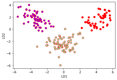
Plotting LDA components:

plt.xlabel('LD1')
plt.ylabel('LD2')
plt.scatter(lda_t[:,0],lda_t[:,1],c=y,cmap='rainbow',edgecolors='r')

LDA for classification:

X_train,X_test,y_train,y_test = train_test_split(X,y,test_size=0.3)
lda.fit(X_train,y_train)

Accuracy Score:

y_pred = lda.predict(X_test)
print(accuracy_score(y_test,y_pred))

Confusion Matrix:

confusion_matrix(y_test,y_pred)

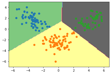
Plotting Decision boundary for our dataset:

min1,max1 = lda_t[:,0].min()-1, lda_t[:,0].max()+1
min2,max2 = lda_t[:,1].min()-1,lda_t[:,1].max()+1
x1grid = np.arange(min1,max1,0.1)
x2grid = np.arange(min2,max2,0.1)
xx,yy = np.meshgrid(x1grid,x2grid)
r1,r2 = xx.flatten(),yy.flatten()
r1,r2 = r1.reshape((len(r1),1)), r2.reshape((len(r2),1))
grid = np.hstack((r1,r2))

model = LinearDiscriminantAnalysis()
model.fit(lda_t,y)
yhat = model.predict(grid)
zz = yhat.reshape(xx.shape)
plt.contourf(xx,yy,zz,cmap='Accent')

for class_value in range(3):
  row_ix = np.where( y== class_value)
  plt.scatter(lda_t[row_ix,0],lda_t[row_ix,1])

Conclusion

Linear Discriminant Analysis (LDA) stands out as a valuable tool for simplifying data and making classifications. We’ve covered why LDA is important, its limitations, and key components such as Fisher’s Linear Discriminant. Understanding the numerator and denominator in LDA, its application for multiple classes, and its implementation in Python provides practical insights. Recognizing and addressing LDA’s limitations is crucial for effective use in diverse scenarios.

Key Takeaways:

• LDA maximizes between-class scatter while minimizing within-class scatter
• It assumes Gaussian distribution and identical covariance matrices for classes
• LDA can be extended for multi-class problems and addresses some limitations of logistic regression
• Regularization techniques help overcome LDA’s small sample size problem

The media shown in this article are not owned by Analytics Vidhya and are used at the Author’s discretion.

Frequently Asked Questions

Sunil Kumar Dash 27 Jun, 2024