A Walk-through of Regression Analysis Using Artificial Neural Networks in Tensorflow

This article was published as a part of the Data Science Blogathon

Linear Regression

Linear Regression is a supervised learning technique that involves learning the relationship between the features and the target. The target values are continuous, which means that the values can take any values between an interval. For example, 1.2, 2.4, and 5.6 are considered to be continuous values. Use-cases of regression include stock market price prediction, house price prediction, sales prediction, and etc.

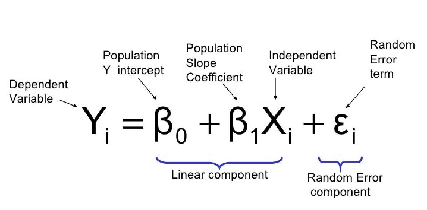
The y hat is called the hypothesis function. The objective of linear regression is to learn the parameters in the hypothesis function. The model parameters are, intercept (beta 0) and the slope (beta 1). The above equation is valid for univariate data, which means there is only one column in the data as a feature.

How does linear regression learn the parameters?

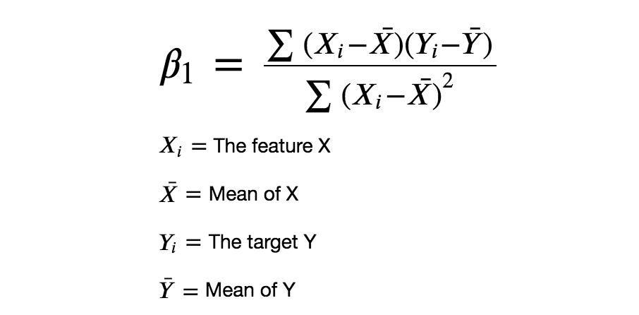
The numerator denotes the covariance of the data and the denominator denotes the variance of the feature X. The result will be the value of beta 1 which is also called the slope. The beta 1 parameter determines the slope of the linear regression line. The intercept decides where the line should pass through in the y-axis.

 

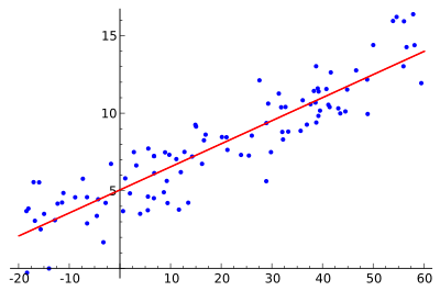
In the image above the intercept-value would be 5, because it is the point where the linear regression line passes through the y-axis. In this way, the linear regression learns the relationship between the features and target.

Regression using Artificial Neural Networks

Why do we need to use Artificial Neural Networks for Regression instead of simply using Linear Regression?

The purpose of using Artificial Neural Networks for Regression over Linear Regression is that the linear regression can only learn the linear relationship between the features and target and therefore cannot learn the complex non-linear relationship. In order to learn the complex non-linear relationship between the features and target, we are in need of other techniques. One of those techniques is to use Artificial Neural Networks. Artificial Neural Networks have the ability to learn the complex relationship between the features and target due to the presence of activation function in each layer. Let’s look at what are Artificial Neural Networks and how do they work.

Artificial Neural Networks

Artificial Neural Networks are one of the deep learning algorithms that simulate the workings of neurons in the human brain. There are many types of Artificial Neural Networks, Vanilla Neural Networks, Recurrent Neural Networks, and Convolutional Neural Networks. The Vanilla Neural Networks have the ability to handle structured data only, whereas the Recurrent Neural Networks and Convolutional Neural Networks have the ability to handle unstructured data very well. In this post, we are going to use Vanilla Neural Networks to perform the Regression Analysis.

Structure of Artificial Neural Networks

 

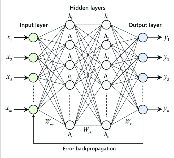
The Artificial Neural Networks consists of the Input layer, Hidden layers, Output layer. The hidden layer can be more than one in number. Each layer consists of n number of neurons. Each layer will be having an Activation Function associated with each of the neurons. The activation function is the function that is responsible for introducing non-linearity in the relationship. In our case, the output layer must contain a linear activation function. Each layer can also have regularizers associated with it. Regularizers are responsible for preventing overfitting.

Artificial Neural Networks consists of two phases,

• Forward Propagation
• Backward Propagation

Forward propagation is the process of multiplying weights with each feature and adding them. The bias is also added to the result. Backward propagation is the process of updating the weights in the model. Backward propagation requires an optimization function and a loss function.

Regression Analysis Using Tensorflow

The entire code was executed in Google Colab. The data we use is the California housing prices dataset, in which we are going to predict the median housing prices. The data is available in the Colab in the path /content/sample_data/california_housing_train.csv. We are going to use TensorFlow to train the model.

Import the required libraries.

import math
import pandas as pd
import tensorflow as tf
import matplotlib.pyplot as plt
from tensorflow.keras import Model
from tensorflow.keras import Sequential
from tensorflow.keras.optimizers import Adam
from sklearn.preprocessing import StandardScaler
from tensorflow.keras.layers import Dense, Dropout
from sklearn.model_selection import train_test_split
from tensorflow.keras.losses import MeanSquaredLogarithmicError
TRAIN_DATA_PATH = '/content/sample_data/california_housing_train.csv'
TEST_DATA_PATH = '/content/sample_data/california_housing_test.csv'
TARGET_NAME = 'median_house_value'

The training data is in the path /content/sample_data/california_housing_train.csv and the test data is in the path /content/sample_data/california_housing_test.csv in Google Colab. The target name in the data is median_house_value.

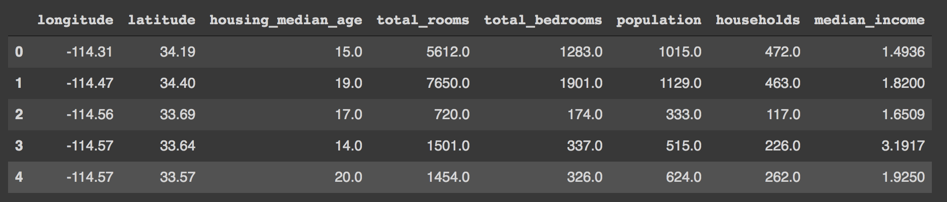
# x_train = features, y_train = target
train_data = pd.read_csv(TRAIN_DATA_PATH)
test_data = pd.read_csv(TEST_DATA_PATH)
x_train, y_train = train_data.drop(TARGET_NAME, axis=1), train_data[TARGET_NAME]
x_test, y_test = test_data.drop(TARGET_NAME, axis=1), test_data[TARGET_NAME]

Read the train and test data and split the data into features and targets. The x_train would look like the following image.

 

def scale_datasets(x_train, x_test):

  """
  Standard Scale test and train data
  Z - Score normalization
  """
  standard_scaler = StandardScaler()
  x_train_scaled = pd.DataFrame(
      standard_scaler.fit_transform(x_train),
      columns=x_train.columns
  )
  x_test_scaled = pd.DataFrame(
      standard_scaler.transform(x_test),
      columns = x_test.columns
  )
  return x_train_scaled, x_test_scaled
x_train_scaled, x_test_scaled = scale_datasets(x_train, x_test)

The function scale_datasets is used to scale the data. Scaling the data would result in faster convergence to the global optimal value for loss function optimization functions. Here we use Sklearn’s StandardScaler class which performs z-score normalization. The z-score normalization subtracts each data from its mean and divides it by the standard deviation of the data. We are going to train with the scaled dataset.

hidden_units1 = 160
hidden_units2 = 480
hidden_units3 = 256
learning_rate = 0.01
# Creating model using the Sequential in tensorflow
def build_model_using_sequential():
  model = Sequential([
    Dense(hidden_units1, kernel_initializer='normal', activation='relu'),
    Dropout(0.2),
    Dense(hidden_units2, kernel_initializer='normal', activation='relu'),
    Dropout(0.2),
    Dense(hidden_units3, kernel_initializer='normal', activation='relu'),
    Dense(1, kernel_initializer='normal', activation='linear')
  ])
  return model
# build the model
model = build_model_using_sequential()

We are going to build the Neural Network model using TensorFlow’s Sequential class. Here we have used four layers. The first layer consists of 160 hidden units/ neurons with the ReLU activation function. ReLU stands for Rectified Linear Units. The second layer consists of 480 hidden units with the ReLU activation function. The third layer consists of 256 hidden units with the ReLU activation function. The final layer is the output layer which consists of one unit with a linear activation function.

# loss function
msle = MeanSquaredLogarithmicError()
model.compile(
    loss=msle, 
    optimizer=Adam(learning_rate=learning_rate), 
    metrics=[msle]
)
# train the model
history = model.fit(
    x_train_scaled.values, 
    y_train.values, 
    epochs=10, 
    batch_size=64,
    validation_split=0.2
)

After building the model with the Sequential class we need to compile the model with training configurations. We use Mean Squared Logarithmic Loss as loss function and metric, and Adam loss function optimizer. The loss function is used to optimize the model whereas the metric is used for our reference. After compiling the model we need to train the model. For training, we use the function fit which takes in the following parameters, features, target, epochs, batch size, and validation split. We have chosen 10 epochs to run. An epoch is a single pass through the training data. A batch size of 64 is used.

 

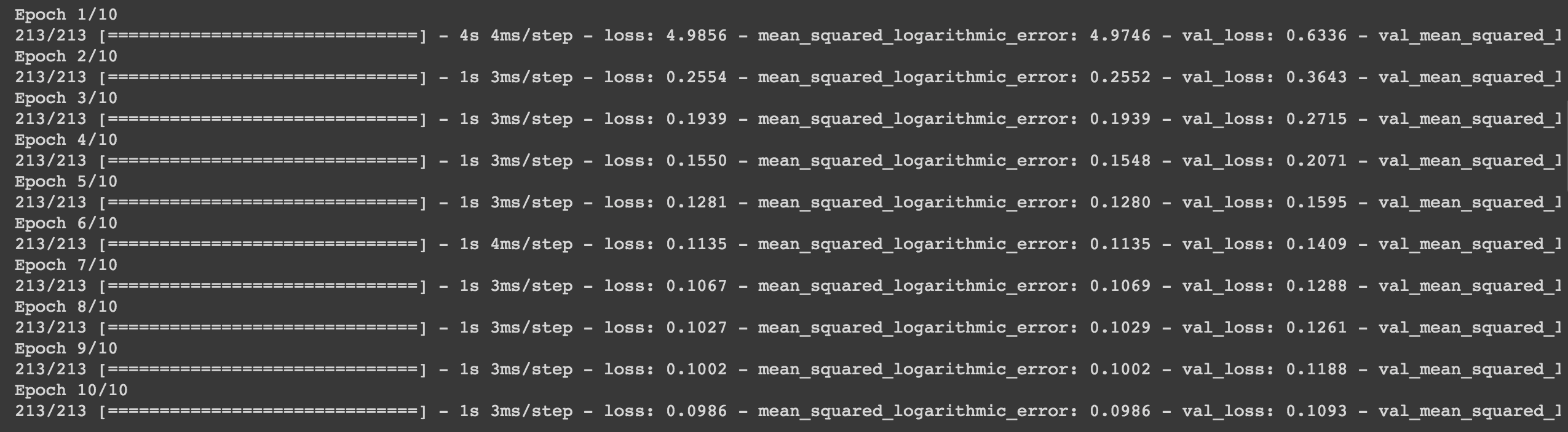
After training, plot the history.

def plot_history(history, key):
  plt.plot(history.history[key])
  plt.plot(history.history['val_'+key])
  plt.xlabel("Epochs")
  plt.ylabel(key)
  plt.legend([key, 'val_'+key])
  plt.show()
# Plot the history
plot_history(history, 'mean_squared_logarithmic_error')

 

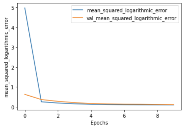
The image above shows that as the epochs increase the loss decreases, which is a good sign of progress. Now that we have trained the model, we can use that model to predict the unseen data, in our case, the test data.

x_test['prediction'] = model.predict(x_test_scaled)

 

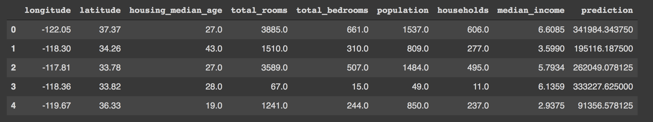
In this way, you can utilize Artificial Neural Networks to perform Regression Analysis.

Frequently Asked Questions

Summary

• Read the California housing price dataset
• Split the data into features and target
• Scale the dataset using z-score normalization
• Train the Neural Network model with four layers, Adam optimizer, Mean Squared Logarithmic Loss, and a batch size of 64.
• After training, plot the history of epochs
• Predict the test data using the trained model

In this post, we have learned to train a Neural Network model to perform Regression analysis. Never hold yourself back to change the hyperparameters in the model.

The hyperparameters we have used are, activation function, number of layers, number of hidden units in a layer, optimization function, batch size, and epochs.

Happy Deep Learning!

Connect with me on LinkedIn.

The media shown in this article are not owned by Analytics Vidhya and are used at the Author’s discretion.

Srivignesh R 18 Jul 2023

Machine Learning Engineer @ Zoho Corporation