PCA And It’s Underlying Mathematical Principles
This article was published as a part of the Data Science Blogathon
Introduction
In this article we will try to understand what PCA is all about, why do we need to perform PCA on a given dataset. We also look into the Mathematical Principles or the concepts underlying PCA and how these concepts help us in determining the Principal Components for a given dataset. Finally, we will look into the steps involved in performing PCA using the Air Quality Index dataset using Python as a tool.
Before, getting into what PCA is all about and the steps involved in it. First, let us try to understand why do we need to perform PCA as part of any Data Science Project especially when we have a large dataset involved.
CONTENTS:
- Why PCA and Why Dimensionality Reduction?:
- Mathematical Concepts Underlying PCA:
- Steps Involved In PCA:
- Scree Plot to decide on the Number of Principal Components:
- Advantages and Limitations of PCA.
Why PCA and why Dimensionality Reduction?
Imagine we have a large dataset, which has multiple dimensions or features. Just by looking at it and trying to perform EDA and analyzing the hidden patterns in the data is a tedious job and for a naked human eye, it is next to impossible to try to understand hidden patterns just by looking at the data.
This is where the PCA comes to our rescue. The idea behind PCA is simply to find a low-dimension set of axes that summarize data. Why do we need to summarize the data though?
Let us try to understand why do we need to summarize the data by taking an example. We have a dataset composed of a set of properties from Laptops. These properties describe each Laptop by its size, color, screen size, weight, processor, number of USB slots, O.S., Touch screen or no Touch screen, and so on. However, many of those features will measure related properties and thus are going to be redundant. Therefore, we should remove this redundancy and describe each laptop with fewer properties. This is exactly what PCA does.
For example, think about the screen size as a feature of Laptops, almost every example has a screen size almost similar, hence we can conclude that this feature has a low variance (On average, most popular laptops have screen sizes that range between 13 to 15 inches.), so this feature will make all laptops look the same, but they are pretty different from each other.
Now, consider the processor as a feature, which has different values (generations) for it, the variance has a great range from the lowest processor generation up to the latest processor. The processor of these laptops is a good property to separate them.
So, here we need to understand the concept very clearly, do not think that PCA is just dropping the feature of the screen size of Laptops and thus by considering the processor feature and other features which has significant variance in it is reducing the dimensions of the given dataset. NO. PCA does not drop any feature present in the original dataset and arrives at Principal Components.
The Algorithm actually constructs a new set of properties which is a combination of the old ones. Mathematically speaking, PCA performs a Linear Transformation moving the original set of features to a new space composed by the Principal Component. These new features do not have any real meaning except algebraic, therefore do not think that by combining features, linearly you will find new features that you have never thought could exist.
How does the new PCA space look like?
In the new feature space, we are trying to find some properties that strongly differ across the classes. As discussed in the above example, some properties that present low variance are not useful, it will make the laptops look the same. On the other hand, PCA looks for properties that show the maximum amount of variation across classes as possible to create the Principal Component Space. The algorithm uses the concepts of Variance Matrix, Covariance Matrix, Eigenvector, and EigenValues pairs to perform PCA, providing a set of eigenvectors and its respective eigenvalues as a result.
The concepts of Covariance Matrix, Eigenvalues, and Eigenvectors are explained in the section below on Mathematical concepts behind PCA.
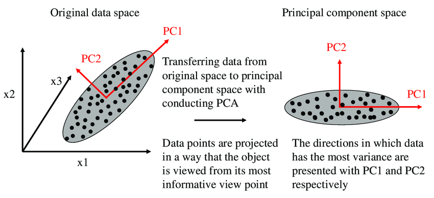
IMAGE 1
Mathematical Concepts underlying PCA
It is important for us to understand the Mathematical concepts underlying PCA for a better understanding of PCA as a whole and also how these concepts help us in determining the Principal Components for a given dataset.
What should we do with Eigenvalues and Eigenvectors? why are they computed? The answer to these questions is simple; the Eigenvectors represent the new set of axes of the Principal component space and also the Eigenvalues carry the information of the amount of variance that each eigenvector has. So to scale back the dimensions of the dataset we are going to choose those Eigenvectors that have more variance and discard those with less variance.
Now, let us look at Covariance Matrix and how does it help us in computing the Principal Components.
Covariance and Variance are a measure of the “spread” of a set of points around their center of mass(mean).
Covariance is measured between 2 dimensions to see if there is a relationship between the 2 dimensions e.g. number of hours studied and marks obtained.
The following is the Mathematical Formula for covariance.

So, if you had a 3-dimensional dataset (X, Y, Z), then you’ll measure the covariance between the X and Y dimensions, the Y and Z dimensions, and also the X and Z dimensions. Measuring the covariance between X and X, or Y and Y, or Z and Z would give you the variance of the X, Y, and Z dimensions respectively.
Covariance Matrix represents Covariance between dimensions as a Matrix ex: for 3 dimensions: Cov(X, X) Cov(X,Y) and Cov(X,Z).
The covariance Matrix is symmetrical about its diagonal.
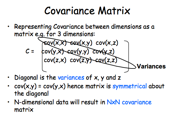
IMAGE 2
Now, let us move onto the next section of our article about how PCA is performed on a given dataset and the steps involved in performing the PCA. We will perform the PCA on the Air Quality Index dataset and try to find out which Principal Components would be required for further analysis. Our original dataset has 16 columns or features and 2009 entries or records. We will perform PCA on this dataset.
Let’s also try to understand why each step becomes important in performing PCA and how it is helping in determining the final Principal Components for a given dataset and the Mathematical concepts involved in each step:
Steps Involved in PCA
1. Standardization of the continuous variables of the dataset.
2. Computing the Co-variance Matrix to identify Co-relations.
3. Computing the Eigen Values and Eigenvectors of the covariance Matrix to identify the Principal Components.
4. Deciding on the Principal Components to be kept for further analysis based on the variation in the Components using the Scree Plot.
5. Recast the data along the Principal Component’s axes.
Let’s now discuss each step in detail:
Step 1: Standardization
Let us first try to understand why do we need to perform Standardization of the continuous variables before performing PCA.
The reason why it is important to perform standardization before PCA is that the latter is extremely sensitive regarding the variances of the variables. i.e. if there are large differences between the ranges of initial variables, those variables with larger ranges will dominate over those with small ranges(For example, a variable that ranges between 0 and 100 will dominate over a variable that ranges between 0 and 1), which can cause biased results. So transforming the data to comparable scales will prevent this problem.
The following is the code to perform Standardization on the given dataset using Python.
from scipy.stats import zscore
df_num_scaled=df_num.apply(zscore)
df_num_scaled.head()
Statistical Tests to be done for PCA
The following are the 2 tests that we perform on the dataset to identify whether to perform PCA on the given dataset or not to perform the same.
1. Bartlett’s Test of Sphericity
2. The Kaiser- Meyer- Olkin (KMO) – a Measure of Sampling Adequacy (MSA)
Bartlett’s Test of Sphericity: It tests the hypothesis that the variables are uncorrelated within the population.
H0: Null Hypothesis: All variables in the data are uncorrelated.
Ha: Alternate Hypothesis: At least one pair of variables in the data are correlated if the null hypothesis cannot be rejected, then PCA is not advisable.
If the p-value is small, then we can reject the Null Hypothesis and agree that there is at least one pair of variables in the data which are correlated hence PCA is recommended.
The Kaiser- Meyer- Olkin (KMO) – a Measure of Sampling Adequacy (MSA) is an index used to determine how appropriate PCA is. Generally, if MSA is less than 0.5, PCA is not recommended, since no reduction is expected. On the other hand, MSA>0.7 is expected to provide a considerable reduction in the dimension and extraction of meaningful components.
Now, let us perform the above two tests on our dataset.
The following is the code for performing Bartlett’s Test of Sphericity:
from factor_analyzer.factor_analyzer import calculate_bartlett_sphericity
chi_square_value,p_value=calculate_bartlett_sphericity(df_num_scaled)
p_value
OUTPUT: 0.0
For our dataset p_value is 0.0 which is less than 0.05. Hence we can reject the Null Hypothesis and agree that there is at least one pair of variables in the data which are correlated. Hence, PCA is recommended.
Now, let us perform The Kaiser- Meyer- Olkin (KMO)- test on the given dataset.
The following is the code for KMO – test:
from factor_analyzer.factor_analyzer import calculate_kmo
kmo_all,kmo_model=calculate_kmo(df_num_scaled)
kmo_model
Output:
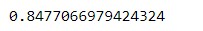
For our dataset MSA value is 0.8477 (by considering four decimal points) which is higher than 0.7. Hence, performing PCA on our dataset is expected to provide a considerable reduction in the dimension and extraction of meaningful components.
Step 2: Covariance Matrix Computation
In this step, we will try to identify if there is any relationship between the variables in the dataset. As sometimes, variables are highly correlated in a way such that the information contained in them is redundant. So as to identify these co-relations, we compute the Covariance Matrix.
The following is the code for computing Covariance Matrix using Python:
cov_matrix = np.cov(df_num_scaled.T)
print('Covariance Matrix n%s', cov_matrix)

STEP 3: Computing Eigenvectors and Eigenvalues
Eigenvectors and Eigenvalues are the Mathematical Concepts of Linear Algebra that we’ve to calculate from the Covariance Matrix to find out the Principal Components of the dataset. Let’s first try and understand what exactly is Principal Components are before actually computing them.
Mathematically speaking, Principal Components represent the directions of the data that specify a maximum amount of variance i.e. the lines that capture most information present in the data.
To put it in a simpler way, just consider Principal Components as new axes that provide the best angle to visualize and evaluate the data, in order that the difference between the observations is best visible.
The following is the code for computing Eigen Values and Eigen Vectors:
eig_vals, eig_vecs = np.linalg.eig(cov_matrix)
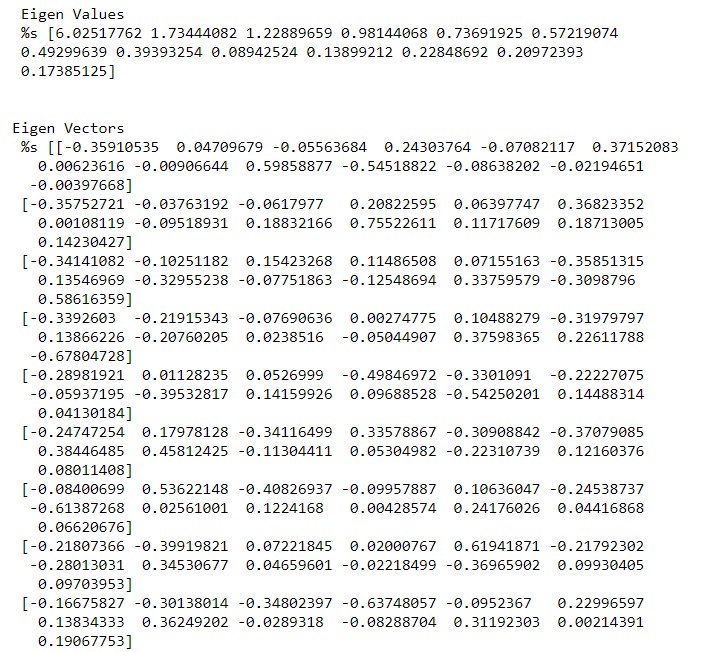
print('n Eigen Values n %s', eig_vals)
print('n')
print('Eigen Vectors n %s', eig_vecs)
EIGENVALUES EIGEN VECTORS
The following is the code for Cumulative Variance explained.
tot = sum(eig_vals)
var_exp = [( i /tot ) * 100 for i in sorted(eig_vals, reverse=True)]
cum_var_exp = np.cumsum(var_exp)
print("Variance Explainedn", var_exp)
print("n")
print("Cumulative Variance Explainedn", cum_var_exp)
OUTPUT:
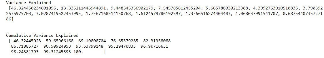
For our dataset, from the above output, we can see that the cumulative variance explained for the 5 components is around 82.3195 percent. So in general we will consider the Principal Components up until 80 to 85 percent of the variance. However, the number of Principal Components to be selected for further analysis depends on the Business problem which we are trying to solve. However, in this case, study, let us consider the first 5 principal components which are explaining around 82% of the variance of the dataset.
Thus, after performing PCA we have actually reduced the dimensions of the dataset from 16 features initially to 5 Principal components which are useful for further analysis as it is explaining around 82% of the variation in the dataset.
Step 4: Scree Plot to decide on the Number of PCS
Before actually plotting the Scree plot we will try to understand what the Scree plot is and how does it help us in deciding the number of Principal Components.
A Scree plot always displays the Eigenvalues in a downward curve, ordering the eigenvalues from largest to smallest. According to the Scree test, the ”elbow” of the graph where the Eigenvalues seem to level off is found and factors or components to the left of this point should be retained as significant.
The Scree Plot is used to determine the number of Principal Components to keep in a Principal Component Analysis(PCA).
The following is the code for plotting the Scree Plot:
plt.figure(figsize=(12,7))
sns.lineplot(y=var_exp,x=range(1,len(var_exp)+1),marker='o')
plt.xlabel('Number of Components',fontsize=15)
plt.ylabel('Variance Explained',fontsize=15)
plt.title('Scree Plot',fontsize=15)
plt.grid()
plt.show()

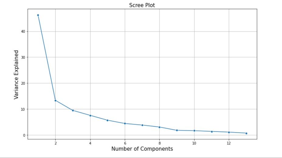
SCREE PLOT OF THE AIR QUALITY INDEX DATASET
From the above Scree Plot, we can see that it is basically an elbow-shaped graph. Where in for our dataset up until 5 Principal Components there is a significant variation or change in the variance explained. Post which it is almost a constant or there is no significant variation. So this by looking at the Scree Plot we can consider the number of Principal Components to be 5 for our dataset. However, as explained above the number of Principal Components to be selected largely depends on the business problem which we are trying to solve.
Step 5: Recasting the Data along with Principal Component Axes
In this step, we are going to use the feature vector formed using the Eigenvectors of the Covariance Matrix, to reorient the data from the original axes to the ones represented by the Principal Components. (Hence the name Principal Component Analysis).
# Using scikit learn PCA here. It does all the above steps and maps data to PCA dimensions in oneshot
from sklearn.decomposition import PCA
# NOTE - we are generating only 5 PCA dimensions (dimensionality reduction from 16 to 5)
pca = PCA(n_components=5, random_state=123)
df_pca = pca.fit_transform(df_num_scaled)
df_pca.transpose() # Component output
Let’s identify which features have Maximum loading across the components. We will first plot the component loading on a heatmap.
For each feature, we find the maximum loading value across the components and mark the same with the help of a rectangular box.
Features marked with the rectangular red boxes are the ones having maximum loading on the respective component. We consider these marked features to decide the context that the component represents.
Code for plotting the Heatmap is as below:
from matplotlib.patches import Rectangle
fig,ax = plt.subplots(figsize=(22, 10), facecolor='w', edgecolor='k')
ax = sns.heatmap(df_pca_loading, annot=True, vmax=1.0, vmin=0, cmap='Blues', cbar=False, fmt='.2g', ax=ax,
                 yticklabels=['PC0','PC1','PC2','PC3','PC4'])
column_max = df_pca_loading.abs().idxmax(axis=0)
for col, variable in enumerate(df_pca_loading.columns):
    position = df_pca_loading.index.get_loc(column_max[variable])
    ax.add_patch(Rectangle((col, position),1,1, fill=False, edgecolor='red', lw=3))
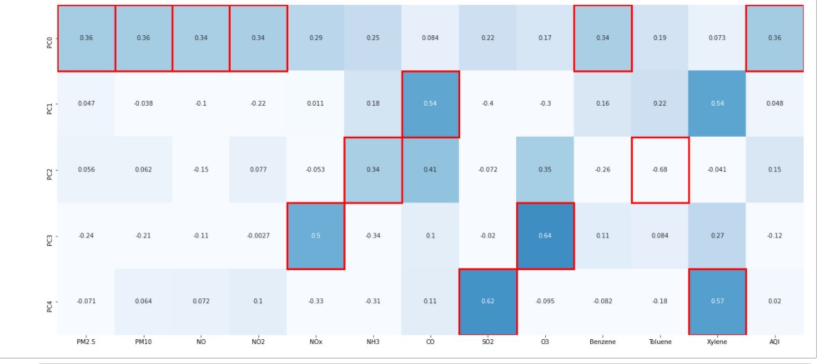
From the above Heat Map, we can see that Principal Component 1(PC0) is a Linear Combination of features P.M. 2.5, P.M. 10, NO, NO2, Benzene. Similarly, the Principal Component 3 (PC2) is a Linear Combination of NH3, Toulene, and so on.
Finally, let us look at some of the Advantages and Limitations of PCA:
Advantages of PCA:
1. Removes correlated Features.
2. Improves Algorithm Performance
3. Reduces Overfitting
4. Improves visualization of the data.
Limitations of PCA:
1. Model Performance: PCA can lead to a reduction in Model Performance on datasets with no or low feature co-relation or does not meet the assumptions of linearity.
2. Outliers: PCA is affected by outliers. Hence treating outliers is important before performing PCA.
3. Interpretability: After performing PCA on the dataset original features will turn into Principal Components which is a Linear Combination of the original features. Hence, these principal components are not as readable as the original features.
Summary:
Now, we can conclude that PCA is one of the best techniques with high performance which is widely used in various industries for its efficiency. PCA is the best choice for dimensionality reduction.
Endnotes:
Thanks for reading!!!
I hope you enjoyed reading the article and hope it helped you in understanding the concept of Principal Component Analysis. If you want to share your thoughts, feel free to comment below in the comment section.
About the author
K. SUMANTH
Currently working with ICICI BANK. Pursuing Data Science and Business Analytics course online. I’m very much interested in knowing what Data wants to tell us about a problem and wants to solve business problems using the data. I’m also enthusiastic about learning and implementing new techniques to Solve Business Problems.
Feel free to connect with me on Linked In.
linkedin.com/in/kowligi-sumanth-37455784
References
- Image 1 – www.researchgate.net
- Image 2 – https://i.stack.imgur.com


