Everything you need to Know about Linear Regression!
Introduction
Linear Regression, a foundational algorithm in data science, plays a pivotal role in predicting continuous outcomes. This guide provides an in-depth exploration of Linear Regression, covering its principles, applications, and implementation in Python on a real-world dataset. From understanding simple and multiple linear regression to unveiling its significance, limitations, and practical use cases, this article serves as a comprehensive resource for both beginners and practitioners. Join us on this journey through the intricacies of linear regression, offering insights into its workings and hands-on application. This article is part of the Data Science Blogathon, delivering valuable knowledge for data enthusiasts
This article was published as a part of the Data Science Blogathon.
Table of contents
- What is Linear Regression?
- Simple Linear Regression
- What is the best fit line?
- Cost Function for Linear Regression
- Gradient Descent for Linear Regression
- Why linear regression is important?
- Evaluation Metrics for Linear Regression
- Assumptions of Linear Regression
- Hypothesis in Linear Regression
- Multiple Linear Regression
- Considerations of Multiple Linear Regression
- Multicollinearity
- Overfitting and Underfitting in Linear Regression
- Bias Variance Tradeoff
- Overfitting
- Underfitting:
- Hands-on Coding: Linear Regression Model
- Conclusion
- Frequently Asked Questions
What is Linear Regression?
“Linear regression predicts the relationship between two variables by assuming a linear connection between the independent and dependent variables. It seeks the optimal line that minimizes the sum of squared differences between predicted and actual values. Applied in various domains like economics and finance, this method analyzes and forecasts data trends. It can extend to multiple linear regression involving several independent variables and logistic regression, suitable for binary classification problems
Simple Linear Regression
In a simple linear regression, there is one independent variable and one dependent variable. The model estimates the slope and intercept of the line of best fit, which represents the relationship between the variables. The slope represents the change in the dependent variable for each unit change in the independent variable, while the intercept represents the predicted value of the dependent variable when the independent variable is zero.
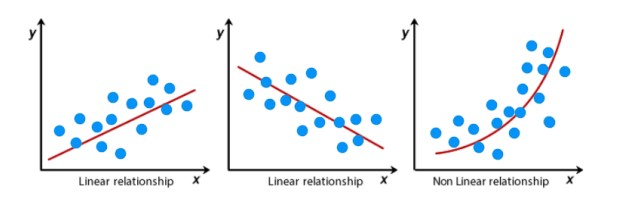
Linear regression is a quiet and the simplest statistical regression method used for predictive analysis in machine learning. Linear regression shows the linear relationship between the independent(predictor) variable i.e. X-axis and the dependent(output) variable i.e. Y-axis, called linear regression. If there is a single input variable X(independent variable), such linear regression is simple linear regression.
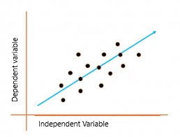
The graph above presents the linear relationship between the output(y) and predictor(X) variables. The blue line is referred to as the best-fit straight line. Based on the given data points, we attempt to plot a line that fits the points the best.
Simple Regression Calculation
To calculate best-fit line linear regression uses a traditional slope-intercept form which is given below,
Yi = β0 + β1Xi
where Yi = Dependent variable, β0 = constant/Intercept, β1 = Slope/Intercept, Xi = Independent variable.
This algorithm explains the linear relationship between the dependent(output) variable y and the independent(predictor) variable X using a straight line Y= B0 + B1 X.
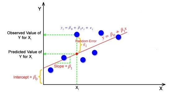
But how the linear regression finds out which is the best fit line?
The goal of the linear regression algorithm is to get the best values for B0 and B1 to find the best fit line. The best fit line is a line that has the least error which means the error between predicted values and actual values should be minimum.
Random Error(Residuals)
In regression, the difference between the observed value of the dependent variable(yi) and the predicted value(predicted) is called the residuals.
εi = ypredicted – yi
where ypredicted = B0 + B1 Xi
What is the best fit line?
In simple terms, the best fit line is a line that fits the given scatter plot in the best way. Mathematically, the best fit line is obtained by minimizing the Residual Sum of Squares(RSS).
Cost Function for Linear Regression
The cost function helps to work out the optimal values for B0 and B1, which provides the best fit line for the data points.
In Linear Regression, generally Mean Squared Error (MSE) cost function is used, which is the average of squared error that occurred between the ypredicted and yi.
We calculate MSE using simple linear equation y=mx+b:

Using the MSE function, we’ll update the values of B0 and B1 such that the MSE value settles at the minima. These parameters can be determined using the gradient descent method such that the value for the cost function is minimum.
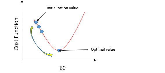
Gradient Descent for Linear Regression
Gradient Descent is one of the optimization algorithms that optimize the cost function(objective function) to reach the optimal minimal solution. To find the optimum solution we need to reduce the cost function(MSE) for all data points. This is done by updating the values of B0 and B1 iteratively until we get an optimal solution.
A regression model optimizes the gradient descent algorithm to update the coefficients of the line by reducing the cost function by randomly selecting coefficient values and then iteratively updating the values to reach the minimum cost function.
Gradient Descent Example
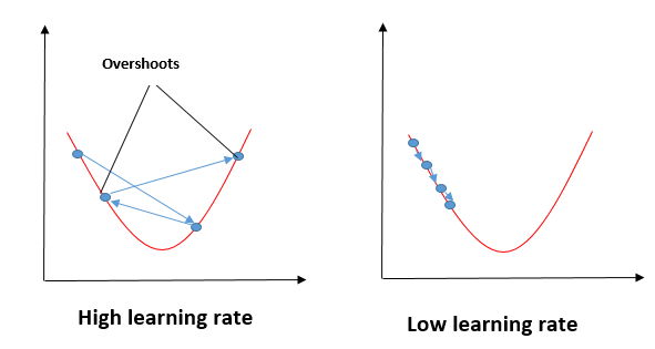
Let’s take an example to understand this. Imagine a U-shaped pit. And you are standing at the uppermost point in the pit, and your motive is to reach the bottom of the pit. Suppose there is a treasure at the bottom of the pit, and you can only take a discrete number of steps to reach the bottom. If you opted to take one step at a time, you would get to the bottom of the pit in the end but, this would take a longer time. If you decide to take larger steps each time, you may achieve the bottom sooner but, there’s a probability that you could overshoot the bottom of the pit and not even near the bottom. In the gradient descent algorithm, the number of steps you’re taking can be considered as the learning rate, and this decides how fast the algorithm converges to the minima.
To update B0 and B1, we take gradients from the cost function. To find these gradients, we take partial derivatives for B0 and B1.
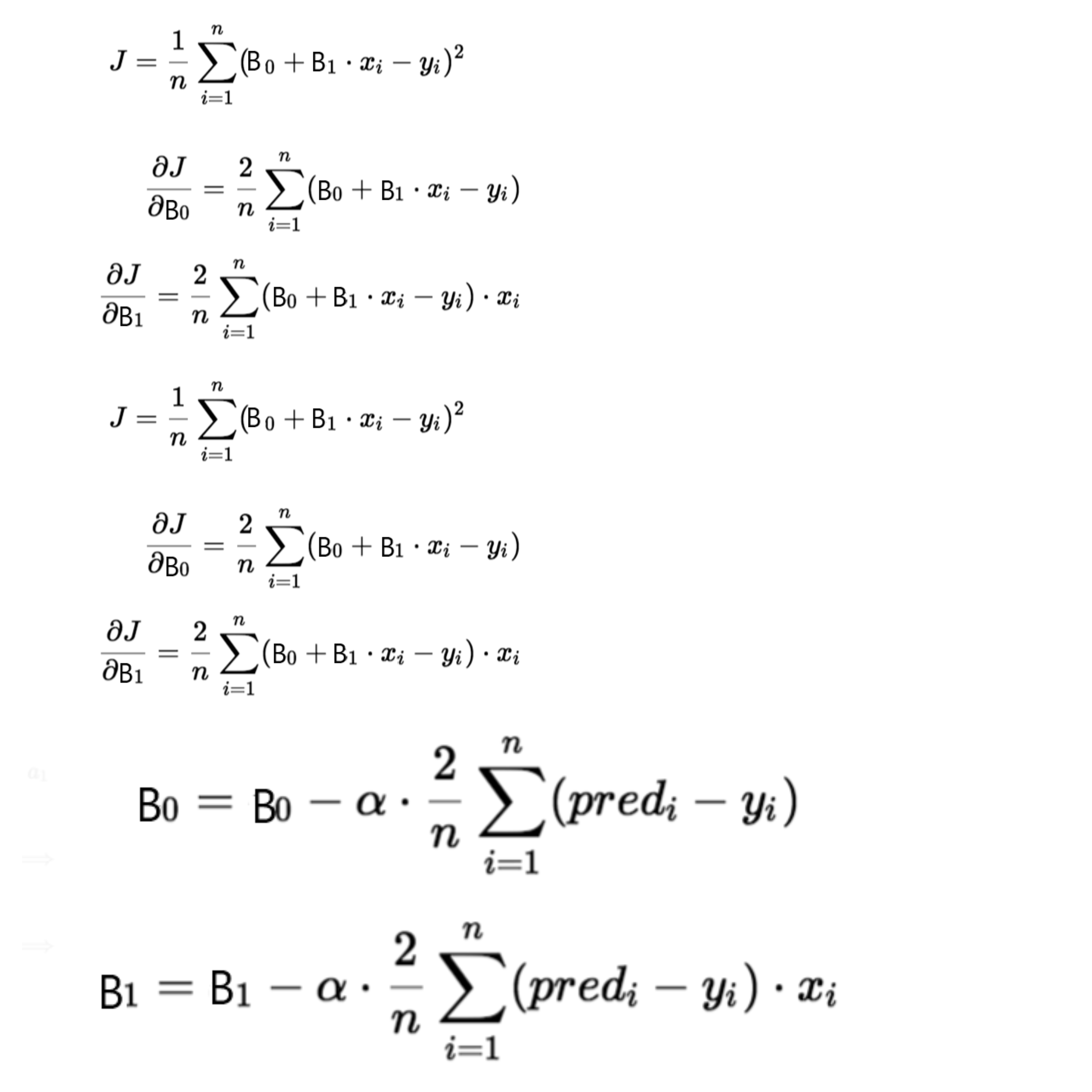
We need to minimize the cost function J. One of the ways to achieve this is to apply the batch gradient descent algorithm. In batch gradient descent, the values are updated in each iteration. (Last two equations shows the updating of values)
The partial derivates are the gradients, and they are used to update the values of B0 and B1. Alpha is the learning rate.
Why linear regression is important?
Linear regression is important for a few reasons:
- Simplicity and interpretability: It’s a relatively easy concept to understand and apply. The resulting model is a straightforward equation that shows how one variable affects another. This makes it easier to explain and trust the results compared to more complex models.
- Prediction: Linear regression allows you to predict future values based on existing data. For instance, you can use it to predict sales based on marketing spend or house prices based on square footage.
- Foundation for other techniques: It serves as a building block for many other data science and machine learning methods. Even complex algorithms often rely on linear regression as a starting point or for comparison purposes.
- Widespread applicability: Linear regression can be used in various fields, from finance and economics to science and social sciences. It’s a versatile tool for uncovering relationships between variables in many real-world scenarios.
In essence, linear regression provides a solid foundation for understanding data and making predictions. It’s a cornerstone technique that paves the way for more advanced data analysis methods.
Evaluation Metrics for Linear Regression
The strength of any linear regression model can be assessed using various evaluation metrics. These evaluation metrics usually provide a measure of how well the observed outputs are being generated by the model.
The most used metrics are,
- Coefficient of Determination or R-Squared (R2)
- Root Mean Squared Error (RSME) and Residual Standard Error (RSE)
Coefficient of Determination or R-Squared (R2)
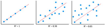
R-Squared is a number that explains the amount of variation that is explained/captured by the developed model. It always ranges between 0 & 1 . Overall, the higher the value of R-squared, the better the model fits the data.
Mathematically it can be represented as,
R2 = 1 – ( RSS/TSS )
- Residual sum of Squares (RSS) is defined as the sum of squares of the residual for each data point in the plot/data. It is the measure of the difference between the expected and the actual observed output.

- Total Sum of Squares (TSS) is defined as the sum of errors of the data points from the mean of the response variable. Mathematically TSS is,
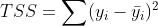
where y hat is the mean of the sample data points.
The significance of R-squared is shown by the following figures,
Root Mean Squared Error
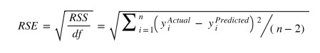
The Root Mean Squared Error is the square root of the variance of the residuals. It specifies the absolute fit of the model to the data i.e. how close the observed data points are to the predicted values. Mathematically it can be represented as,
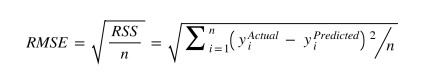
To make this estimate unbiased, one has to divide the sum of the squared residuals by the degrees of freedom rather than the total number of data points in the model. This term is then called the Residual Standard Error(RSE). Mathematically it can be represented as,
R-squared is a better measure than RSME. Because the value of Root Mean Squared Error depends on the units of the variables (i.e. it is not a normalized measure), it can change with the change in the unit of the variables.
Assumptions of Linear Regression
Regression is a parametric approach, which means that it makes assumptions about the data for the purpose of analysis. For successful regression analysis, it’s essential to validate the following assumptions.
- Linearity of residuals: There needs to be a linear relationship between the dependent variable and independent variable(s).
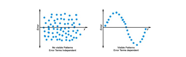
2. Independence of residuals: The error terms should not be dependent on one another (like in time-series data wherein the next value is dependent on the previous one). There should be no correlation between the residual terms. The absence of this phenomenon is known as Autocorrelation.
There should not be any visible patterns in the error terms.
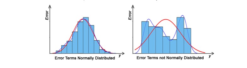
3. Normal distribution of residuals: The mean of residuals should follow a normal distribution with a mean equal to zero or close to zero. This is done in order to check whether the selected line is actually the line of best fit or not.
If the error terms are non-normally distributed, suggests that there are a few unusual data points that must be studied closely to make a better model.
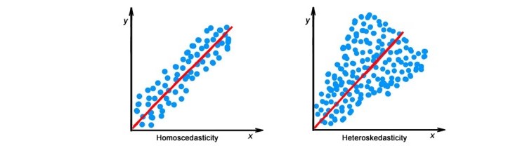
4. The equal variance of residuals: The error terms must have constant variance. This phenomenon is known as Homoscedasticity.
The presence of non-constant variance in the error terms is referred to as Heteroscedasticity. Generally, non-constant variance arises in the presence of outliers or extreme leverage values.
Hypothesis in Linear Regression
Once you have fitted a straight line on the data, you need to ask, “Is this straight line a significant fit for the data?” Or “Is the beta coefficient explain the variance in the data plotted?” And here comes the idea of hypothesis testing on the beta coefficient. The Null and Alternate hypotheses in this case are:
H0: B1 = 0
HA: B1 ≠ 0
To test this hypothesis we use a t-test, test statistics for the beta coefficient is given by,

Assessing the model fit
Some other parameters to assess a model are:
- t statistic: It is used to determine the p-value and hence, helps in determining whether the coefficient is significant or not
- F statistic: It is used to assess whether the overall model fit is significant or not. Generally, the higher the value of the F-statistic, the more significant a model turns out to be.
Multiple Linear Regression
Multiple linear regression is a technique to understand the relationship between a single dependent variable and multiple independent variables.
The formulation for multiple linear regression is also similar to simple linear regression with
the small change that instead of having one beta variable, you will now have betas for all the variables used. The formula is given as:
Y = B0 + B1X1 + B2X2 + … + BpXp + ε
Considerations of Multiple Linear Regression
All the four assumptions made for Simple Linear Regression still hold true for Multiple Linear Regression along with a few new additional assumptions.
- Overfitting: When more and more variables are added to a model, the model may become far too complex and usually ends up memorizing all the data points in the training set. This phenomenon is known as the overfitting of a model. This usually leads to high training accuracy and very low test accuracy.
- Multicollinearity: It is the phenomenon where a model with several independent variables, may have some variables interrelated.
- Feature Selection: With more variables present, selecting the optimal set of predictors from the pool of given features (many of which might be redundant) becomes an important task for building a relevant and better model.
Multicollinearity
As multicollinearity makes it difficult to find out which variable is actually contributing towards the prediction of the response variable, it leads one to conclude incorrectly, the effects of a variable on the target variable. Though it does not affect the precision of the predictions, it is essential to properly detect and deal with the multicollinearity present in the model, as random removal of any of these correlated variables from the model causes the coefficient values to swing wildly and even change signs.
Multicollinearity can be detected using the following methods.
- Pairwise Correlations: Checking the pairwise correlations between different pairs of independent variables can throw useful insights in detecting multicollinearity.
- Variance Inflation Factor (VIF): Pairwise correlations may not always be useful as it is possible that just one variable might not be able to completely explain some other variable but some of the variables combined could be ready to do this. Thus, to check these sorts of relations between variables, one can use VIF. VIF basically explains the relationship of one independent variable with all the other independent variables. VIF is given by,
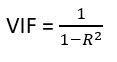
where i refers to the ith variable which is being represented as a linear combination of the rest of the independent variables.
The common heuristic followed for the VIF values is if VIF > 10 then the value is definitely high and it should be dropped. And if the VIF=5 then it may be valid but should be inspected first. If VIF < 5, then it is considered a good vif value.
Overfitting and Underfitting in Linear Regression
There have always been situations where a model performs well on training data but not on the test data. While training models on a dataset, overfitting, and underfitting are the most common problems faced by people.
Before understanding overfitting and underfitting one must know about bias and variance.
Bias:
Bias is a measure to determine how accurate is the model likely to be on future unseen data. Complex models, assuming there is enough training data available, can do predictions accurately. Whereas the models that are too naive, are very likely to perform badly with respect to predictions. Simply, Bias is errors made by training data.
Generally, linear algorithms have a high bias which makes them fast to learn and easier to understand but in general, are less flexible. Implying lower predictive performance on complex problems that fail to meet the expected outcomes.
Variance:
Variance is the sensitivity of the model towards training data, that is it quantifies how much the model will react when input data is changed.
Ideally, the model shouldn’t change too much from one training dataset to the next training data, which will mean that the algorithm is good at picking out the hidden underlying patterns between the inputs and the output variables.
Ideally, a model should have lower variance which means that the model doesn’t change drastically after changing the training data(it is generalizable). Having higher variance will make a model change drastically even on a small change in the training dataset.
Let’s understand what is a bias-variance tradeoff is.
Bias Variance Tradeoff
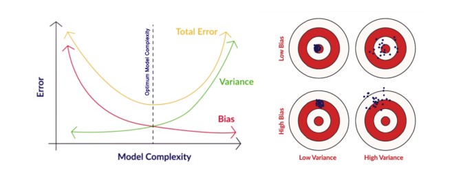
In the pursuit of optimal performance, a supervised machine learning algorithm seeks to strike a balance between low bias and low variance for increased robustness.
In the realm of machine learning, there exists an inherent relationship between bias and variance, characterized by an inverse correlation.
- Increased bias leads to reduced variance.
- Conversely, heightened variance results in diminished bias.
Finding an equilibrium between bias and variance is crucial, and algorithms must navigate this trade-off for optimal outcomes.
In practice, calculating precise bias and variance error terms is challenging due to the unknown nature of the underlying target function.
Now, let’s delve into the nuances of overfitting and underfitting.
Overfitting
When a model learns each and every pattern and noise in the data to such extent that it affects the performance of the model on the unseen future dataset, it is referred to as overfitting. The model fits the data so well that it interprets noise as patterns in the data.
When a model has low bias and higher variance it ends up memorizing the data and causing overfitting. Overfitting causes the model to become specific rather than generic. This usually leads to high training accuracy and very low test accuracy.
Detecting overfitting is useful, but it doesn’t solve the actual problem. There are several ways to prevent overfitting, which are stated below:
- Cross-validation
- If the training data is too small to train add more relevant and clean data.
- If the training data is too large, do some feature selection and remove unnecessary features.
- Regularization
Underfitting:
Underfitting is not often discussed as often as overfitting is discussed. When the model fails to learn from the training dataset and is also not able to generalize the test dataset, is referred to as underfitting. This type of problem can be very easily detected by the performance metrics.
When a model has high bias and low variance it ends up not generalizing the data and causing underfitting. It is unable to find the hidden underlying patterns from the data. This usually leads to low training accuracy and very low test accuracy. The ways to prevent underfitting are stated below,
- Increase the model complexity
- Increase the number of features in the training data
- Remove noise from the data.
Hands-on Coding: Linear Regression Model
This is the section where you’ll find out how to perform the regression in Python. We will use Advertising sales channel prediction data. You can access the data here.
| TV | Radio | Newspaper | Sales |
| 230.1 | 37.8 | 69.2 | 22.1 |
| 44.5 | 39.3 | 45.1 | 10.4 |
| 17.2 | 45.9 | 69.3 | 12.0 |
| 151.5 | 41.3 | 58.5 | 16.5 |
| 180.8 | 10.8 | 58.4 | 17.9 |
| 8.7 | 48.9 | 75.0 | 7.2 |
| 57.5 | 32.8 | 23.5 | 11.8 |
‘Sales’ is the target variable that needs to be predicted. Now, based on this data, our objective is to create a predictive model, that predicts sales based on the money spent on different platforms for marketing.
Let us straightaway get right down to some hands-on coding to get this prediction done. Please don’t feel overlooked if you do not have experience with Python. In fact, the best way to learn is to get your hands dirty by solving a problem – like the one we are doing.
Step 1: Importing Python Libraries
The first step is to fire up your Jupyter notebook and load all the prerequisite libraries in your Jupyter notebook. Here are the important libraries that we will be needing for this linear regression.
- NumPy (to perform certain mathematical operations)
- pandas (to storethe data in a pandas DataFrames)
- matplotlib.pyplot (you will use matplotlib to plot the data)
In order to load these, just start with these few lines of codes in your first cell:
#Importing all the necessary libraries
import numpy as np
import pandas as pd
import matplotlib.pyplot as plt
# Supress Warnings
import warnings
warnings.filterwarnings('ignore')
The last line of code helps in suppressing the unnecessary warnings.
Step 2: Loading the Dataset
Let us now import data into a DataFrame. A DataFrame is a data type in Python. The simplest way to understand it would be that it stores all your data in tabular format.
#Read the given CSV file, and view some sample records
advertising = pd.read_csv( "advertising.csv" )
advertising.head()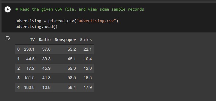
Step 3: Visualization
Let us plot the scatter plot for target variable vs. predictor variables in a single plot to get the intuition. Also, plotting a heatmap for all the variables,
#Importing seaborn library for visualizations
import seaborn as sns
#to plot all the scatterplots in a single plot
sns.pairplot(advertising, x_vars=[ 'TV', ' Newspaper.,'Radio' ], y_vars = 'Sales', size = 4, kind = 'scatter' )
plt.show()#To plot heatmap to find out correlations
sns.heamap( advertising.corr(), cmap = 'YlGnBl', annot = True )
plt.show()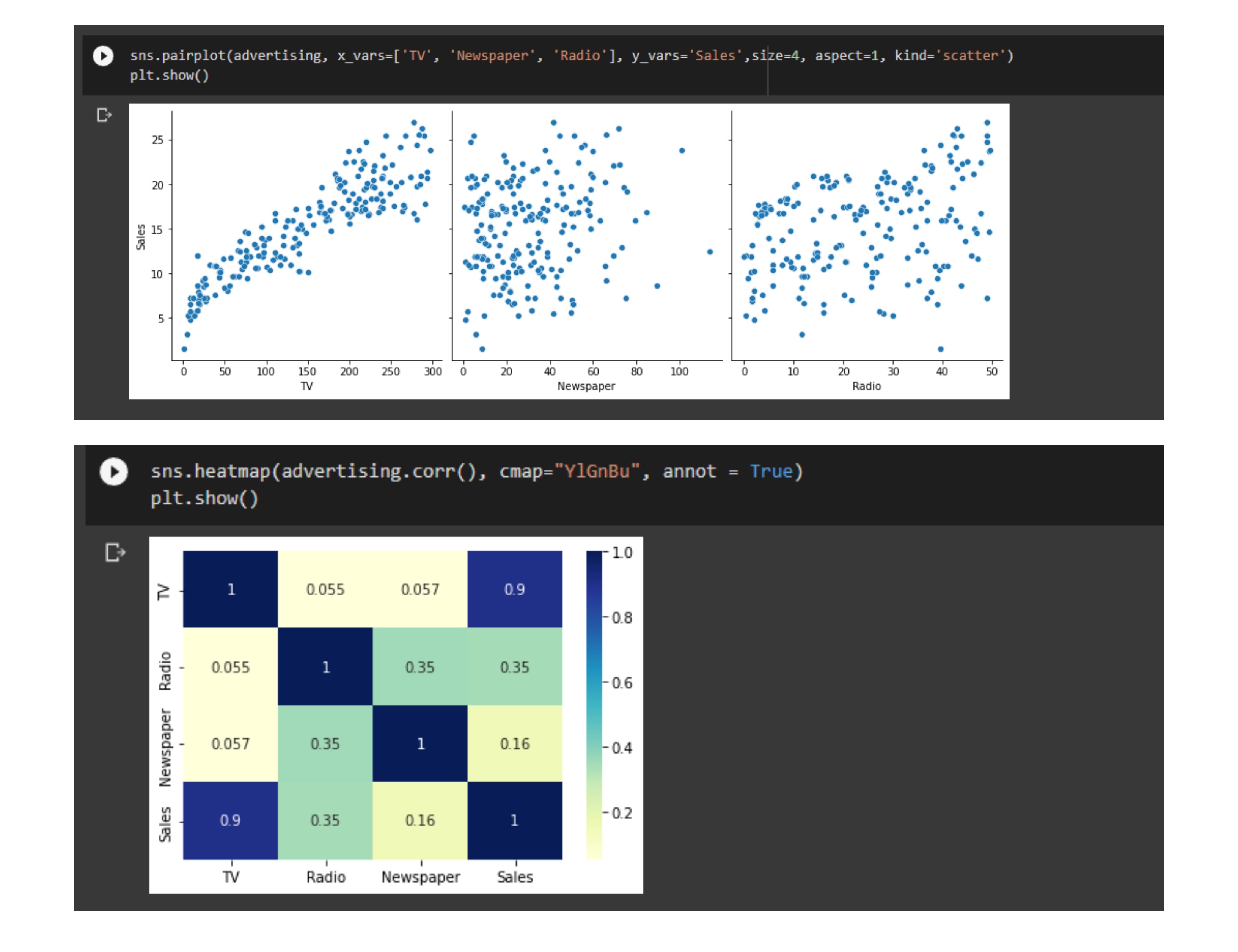
From the scatterplot and the heatmap, we can observe that ‘Sales’ and ‘TV’ have a higher correlation as compared to others because it shows a linear pattern in the scatterplot as well as giving 0.9 correlation.
You can go ahead and play with the visualizations and can find out interesting insights from the data.
Step 4: Performing Simple Linear Regression
Here, as the TV and Sales have a higher correlation we will perform the simple linear regression for these variables.
We can use sklearn or statsmodels to apply linear regression. So we will go ahead with statmodels.
We first assign the feature variable, `TV`, during this case, to the variable `X` and the response variable, `Sales`, to the variable `y`.
X = advertising[ 'TV' ]
y = advertising[ 'Sales' ]
And after assigning the variables you need to split our variable into training and testing sets. You’ll perform this by importing train_test_split from the sklearn.model_selection library. It is usually a good practice to keep 70% of the data in your train dataset and the rest 30% in your test dataset.
from sklearn.model_selection import train_test_split
X_train, X_test, y_train, y_test = train_test_split( X, y, train_size = 0.7, test_size = 0.3, random_state = 100 )
In this way, you can split the data into train and test sets.
One can check the shapes of train and test sets with the following code,
print( X_train.shape )
print( X_test.shape )
print( y_train.shape )
print( y_test.shape )
importing statmodels library to perform linear regression
import statsmodels.api as smBy default, the statsmodels library fits a line on the dataset which passes through the origin. But in order to have an intercept, you need to manually use the add_constant attribute of statsmodels. And once you’ve added the constant to your X_train dataset, you can go ahead and fit a regression line using the OLS (Ordinary Least Squares) the attribute of statsmodels as shown below,
# Add a constant to get an intercept
X_train_sm = sm.add_constant(X_train)
# Fit the resgression line using 'OLS'
lr = sm.OLS(y_train, X_train_sm).fit()
One can see the values of betas using the following code,
# Print the parameters,i.e. intercept and slope of the regression line obtained
lr.params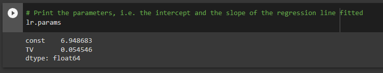
Here, 6.948 is the intercept, and 0.0545 is a slope for the variable TV.
Now, let’s see the evaluation metrics for this linear regression operation. You can simply view the summary using the following code,
#Performing a summary operation lists out all different parameters of the regression line fitted
print(lr.summary())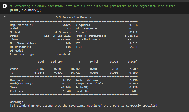
Summary
As you can see, this code gives you a brief summary of the linear regression. Here are some key statistics from the summary:
- The coefficient for TV is 0.054, with a very low p-value. The coefficient is statistically significant. So the association is not purely by chance.
- R – squared is 0.816 Meaning that 81.6% of the variance in `Sales` is explained by `TV`. This is a decent R-squared value.
- F-statistics has a very low p-value(practically low). Meaning that the model fit is statistically significant, and the explained variance isn’t purely by chance.
Step 5: Performing predictions on the test set
Now that you have simply fitted a regression line on your train dataset, it is time to make some predictions on the test data. For this, you first need to add a constant to the X_test data like you did for X_train and then you can simply go on and predict the y values corresponding to X_test using the predict the attribute of the fitted regression line.
# Add a constant to X_test
X_test_sm = sm.add_constant(X_test)
# Predict the y values corresponding to X_test_sm
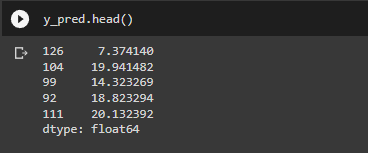
y_pred = lr.predict(X_test_sm)You can see the predicted values with the following code,
y_pred.head()
To check how well the values are predicted on the test data we will check some evaluation metrics using sklearn library.
#Imporitng libraries
from sklearn.metrics import mean_squared_error
from sklearn.metrics import r2_score
#RMSE value
print( "RMSE: ",np.sqrt( mean_squared_error( y_test, y_pred ) )
#R-squared value
print( "R-squared: ",r2_score( y_test, y_pred ) )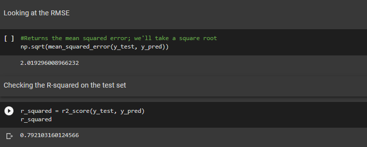
We are getting a decent score for both train and test sets.
Apart from `statsmodels`, there is another package namely `sklearn` that can be used to perform linear regression. We will use the `linear_model` library from `sklearn` to build the model. Since we have already performed a train-test split, we don’t need to do it again.
There’s one small step that we need to add, though. When there’s only a single feature, we need to add an additional column in order for the linear regression fit to be performed successfully. Code is given below,
X_train_lm = X_train_lm.values.reshape(-1,1)
X_test_lm = X_test_lm.values.reshape(-1,1)
One can check the change in the shape of the above data frames.
print(X_train_lm.shape)
print(X_train_lm.shape)
To fit the model, write the below code,
from sklearn.linear_model import LinearRegression
#Representing LinearRegression as lr (creating LinearRegression object)
lr = LinearRegression()
#Fit the model using lr.fit()
lr.fit( X_train_lm , y_train_lm )
You can get the intercept and slope values with sklearn using the following code,
#get intercept
print( lr.intercept_ )
#get slope
print( lr.coef_ )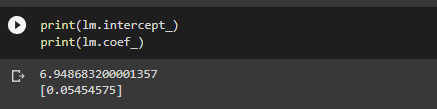
This is how we can perform the simple linear regression.
Conclusion
In conclusion, Linear Regression is a cornerstone in data science, providing a robust framework for predicting continuous outcomes. As we unravel its intricacies and applications, it becomes evident that Linear Regression is a versatile tool with widespread implications. This article is a comprehensive guide from its role in modeling relationships to real-world implementations in Python.
For those eager to delve deeper into the world of data science and machine learning, Analytics Vidhya’s AI & ML BlackBelt+ program offers an immersive learning experience. Elevate your skills and navigate the evolving landscape of data science with mentorship and hands-on projects. Join BB+ today and unlock the next level in your data science journey!
Frequently Asked Questions
A. Linear regression has two main parameters: slope (weight) and intercept. The slope represents the change in the dependent variable for a unit change in the independent variable. The intercept is the value of the dependent variable when the independent variable is zero. The goal is to find the best-fitting line that minimizes the difference between predicted and actual values.
A. The formula for a linear regression line is:
y = mx + b
Where y is the dependent variable, x is the independent variable, m is the slope (weight), and b is the intercept. It represents the best-fitting straight line that describes the relationship between the variables by minimizing the sum of squared differences between actual and predicted values.
Linear regression is used in statistics, economics, finance, and more to analyze relationships between variables. For instance, predicting stock prices in finance or studying the impact of advertising on sales in marketing. A basic example involves predicting weight based on height, where a linear equation is used to estimate weight from height data.
A basic example of linear regression involves predicting a person’s weight based on their height. In this scenario, height is the independent variable, while weight is the dependent variable. The relationship between height and weight is modeled using a simple linear equation, where the weight is estimated as a function of the height.
The media shown in this article are not owned by Analytics Vidhya and are used at the Author’s discretion.


