Understanding Polynomial Regression Model

Hello there, guys! Good day, everyone! Today, we’ll look at Polynomial Regression, a fascinating approach in Machine Learning. For understanding Polynomial Regression Model, we’ll go over several fundamental terms including Machine Learning, Supervised Learning, and the distinction between regression and classification. The topics covered in this comprehensive article are given below.

Table of Contents

• What is Machine Learning?
• Types – Machine Learning
• Supervised Machine Learning
• Classification Vs Regression
• Why do we need Regression?
• Polynomial Regression – Introduction
• Types of Polynomial Regression
• Assumption – Polynomial Regression
• Simple math understanding – Polynomial Regression
• Linear Regression Vs Polynomial Regression
• Non-linear data – Polynomial Regression
• Overfitting Vs Under-fitting
• Bias Vs Variance Tradeoff
• Degree – how to find the right one?
• Cost function – Polynomial Regression
• Gradient Descent – Polynomial Regression
• Practical application of Polynomial Regression
• Application – Polynomial Regression
• Advantage – Polynomial Regression
• Disadvantage – Polynomial Regression

What is Machine Learning?

Machine Learning algorithms may access data (categorical, numerical, image, video, or anything else) and use it to learn for themselves without any explicit programming. But how does Machine Learning function exactly? simply by inspecting the data or facts (through instructions to observe the pattern and making decisions or predictions)

Types of Machine Learning

Algorithmic approaches for machine learning may be divided into three categories.

1. Supervised Machine Learning – Task-Oriented (Classification – Regression)

2. Unsupervised Machine Learning – Fact or Data-Oriented (Cluster – Anomaly detection)

3. Reinforcement Machine Learning – Either learning from mistakes or learning from them correctly

Supervised Machine Learning

In supervised learning, algorithms are trained using labelled datasets, and the algorithm learns about each category of input. The approach is evaluated using test data (a subset of the training set) and predicts the outcome when the training phase is over. Supervised machine learning is classified into two types:

1. Classification

2. Regression

Classification Vs Regression

When there is a link between the input and output variables, regression methods are applied. It is used to forecast continuous variables such as weather and market movements, among others.

Classification methods are employed when the output variable is categorical, such as Yes-No, Male-Female, True-False, Normal – Abnormal, and so on.

Why do we need Regression?

Regression analysis is frequently used for one of two purposes: forecasting the value of the dependent variable for those who have knowledge of the explanatory components, or assessing the influence of an explanatory variable on the dependent variable.

What is Polynomial Regression?

In polynomial regression, the relationship between the independent variable x and the dependent variable y is described as an nth degree polynomial in x. Polynomial regression, abbreviated E(y |x), describes the fitting of a nonlinear relationship between the value of x and the conditional mean of y. It usually corresponded to the least-squares method. According to the Gauss Markov Theorem, the least square approach minimizes the variance of the coefficients. This is a type of Linear Regression in which the dependent and independent variables have a curvilinear relationship and the polynomial equation is fitted to the data; we’ll go over that in more detail later in the article. Machine learning is also referred to as a subset of Multiple Linear Regression. Because we convert the Multiple Linear Regression equation into a Polynomial Regression equation by including more polynomial elements.

Types of Polynomial Regression

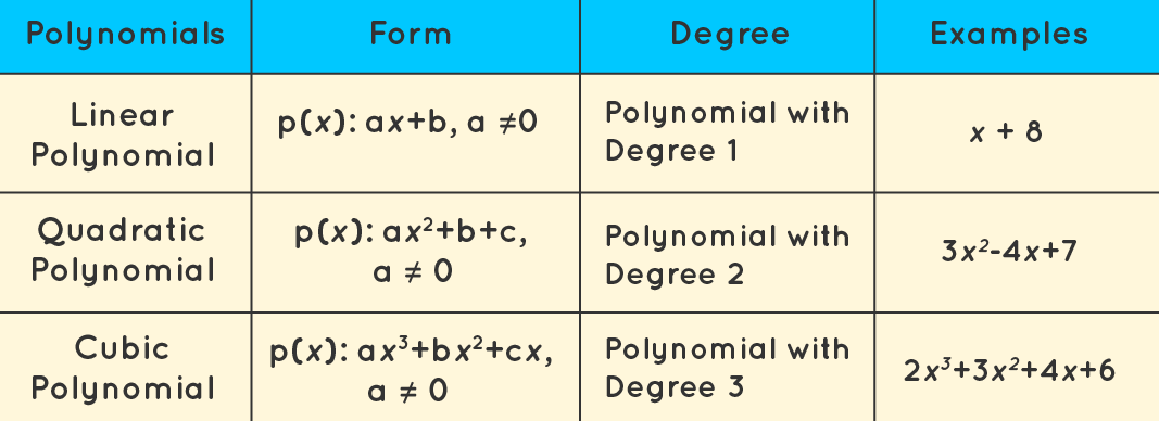
A quadratic equation is a general term for a second-degree polynomial equation. This degree, on the other hand, can go up to nth values. Polynomial regression can so be categorized as follows:

1. Linear – if degree as 1

2. Quadratic – if degree as 2

3. Cubic – if degree as 3 and goes on, on the basis of degree.

Assumption of Polynomial Regression

We cannot process all of the datasets and use polynomial regression machine learning to make a better judgment. We can still do it, but there should be specific constraints for the dataset in order to get the best polynomial regression results.
A dependent variable’s behaviour can be described by a linear, or curved, an additive link between the dependent variable and a set of k independent factors.
The independent variables have no relationship with one another.
We’re utilizing datasets with independent errors that are normally distributed with a mean of zero and a constant variance.

Simple math to understand Polynomial Regression

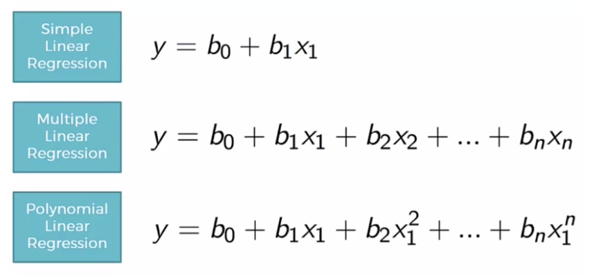
Here we are dealing with mathematics, rather than going deep, just understand the basic structure, we all know the equation of a linear equation will be a straight line, from that if we have many features then we opt for multiple regression just increasing features part alone, then how about polynomial, it’s not about increasing but changing the structure to a quadratic equation, you can visually understand from the diagram,

Linear Regression Vs Polynomial Regression

Rather than focusing on the distinctions between linear and polynomial regression, we may comprehend the importance of polynomial regression by starting with linear regression. We build our model and realize that it performs abysmally. We examine the difference between the actual value and the best fit line we predicted, and it appears that the true value has a curve on the graph, but our line is nowhere near cutting the mean of the points. This is where polynomial regression comes into play; it predicts the best-fit line that matches the pattern of the data (curve).

Python Code:

And now we do regression analysis, in particular, Linear Regression, and see how well our random data gets analyzed perfectly

x = x[:, np.newaxis] y = y[:, np.newaxis] model = LinearRegression()
model.fit(x, y)

y_pred = model.predict(x)
plt.scatter(x, y, s=10)
plt.plot(x, y_pred, color='r')
plt.show()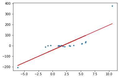

The straight line is unable to capture the patterns in the data, as can be seen. This is an example of under-fitting.

Let’s look at it from a technical standpoint, using measures like Root Mean Square Error (RMSE) and discrimination coefficient (R2). The RMSE indicates how well a regression model can predict the response variable’s value in absolute terms, whereas the R2 indicates how well a model can predict the response variable’s value in percentage terms.

import sklearn.metrics as metrics
mse = metrics.mean_squared_error(x,y)
rmse = np.sqrt(mse) 
r2 = metrics.r2_score(x,y)

print('RMSE value:',rmse)
print('R2 value:',r2)

RMSE value: 93.47170875128153
R2 value: -786.2378753237103

Non-linear data in Polynomial Regression

We need to enhance the model’s complexity to overcome under-fitting. In this sense, we need to make linear analyzes in a non-linear way, statistically by using Polynomial,

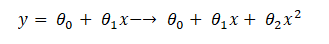
Because the weights associated with the features are still linear, this is still called a linear model. x2 (x square) is only a function. However, the curve we’re trying to fit is quadratic in nature.

Let’s see visually the above concept for better understanding, a picture speaks louder and stronger than words,

from sklearn.preprocessing import PolynomialFeatures
polynomial_features1 = PolynomialFeatures(degree=2)
x_poly1 = polynomial_features1.fit_transform(x)
model1 = LinearRegression()
model1.fit(x_poly1, y)
y_poly_pred1 = model1.predict(x_poly1)

from sklearn.metrics import mean_squared_error, r2_score
rmse1 = np.sqrt(mean_squared_error(y,y_poly_pred1))
r21 = r2_score(y,y_poly_pred1)
print(rmse1)
print(r21)

49.66562739942289
0.7307277801966172

The figure clearly shows that the quadratic curve can better match the data than the linear line.

import operator
plt.scatter(x, y, s=10)
# sort the values of x before line plot
sort_axis = operator.itemgetter(0)
sorted_zip = sorted(zip(x,y_poly_pred), key=sort_axis)
x, y_poly_pred1 = zip(*sorted_zip)
plt.plot(x, y_poly_pred1, color='m')
plt.show()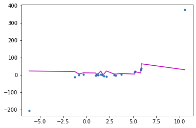

polynomial_features2= PolynomialFeatures(degree=3)
x_poly2 = polynomial_features2.fit_transform(x)
model2 = LinearRegression()
model2.fit(x_poly2, y)
y_poly_pred2 = model2.predict(x_poly2)

rmse2 = np.sqrt(mean_squared_error(y,y_poly_pred2))
r22 = r2_score(y,y_poly_pred2)
print(rmse2)
print(r22)

48.00085922331635
0.7484769902353146

plt.scatter(x, y, s=10)
# sort the values of x before line plot
sort_axis = operator.itemgetter(0)
sorted_zip = sorted(zip(x,y_poly_pred2), key=sort_axis)
x, y_poly_pred2 = zip(*sorted_zip)
plt.plot(x, y_poly_pred2, color='m')
plt.show()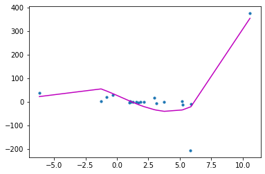

polynomial_features3= PolynomialFeatures(degree=4)
x_poly3 = polynomial_features3.fit_transform(x)
model3 = LinearRegression()
model3.fit(x_poly3, y)
y_poly_pred3 = model3.predict(x_poly3)

rmse3 = np.sqrt(mean_squared_error(y,y_poly_pred3))
r23 = r2_score(y,y_poly_pred3)
print(rmse3)
print(r23)

40.009589710152866
0.8252537381840246

plt.scatter(x, y, s=10)

# sort the values of x before line plot

sort_axis = operator.itemgetter(0)

sorted_zip = sorted(zip(x,y_poly_pred3), key=sort_axis)

x, y_poly_pred3 = zip(*sorted_zip)

plt.plot(x, y_poly_pred3, color='m')

plt.show()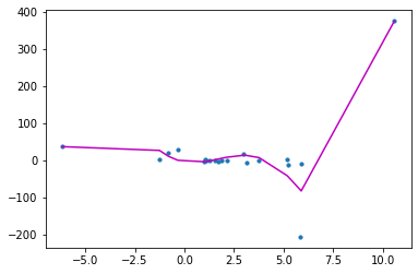

In comparison to the linear line, we can observe that RMSE has dropped and R2-score has increased.

Overfitting Vs Under-fitting

We keep on increasing the degree, we will see the best result, but there comes the over-fitting problem, if we get r2 value for a particular value shows 100.

When analyzing a dataset linearly, we encounter an under-fitting problem, which can be corrected using polynomial regression. However, when fine-tuning the degree parameter to the optimal value, we encounter an over-fitting problem, resulting in a 100 per cent r2 value. The conclusion is that we must avoid both overfitting and underfitting issues.

Note: To avoid over-fitting, we can increase the number of training samples so that the algorithm does not learn the system’s noise and becomes more generalized.

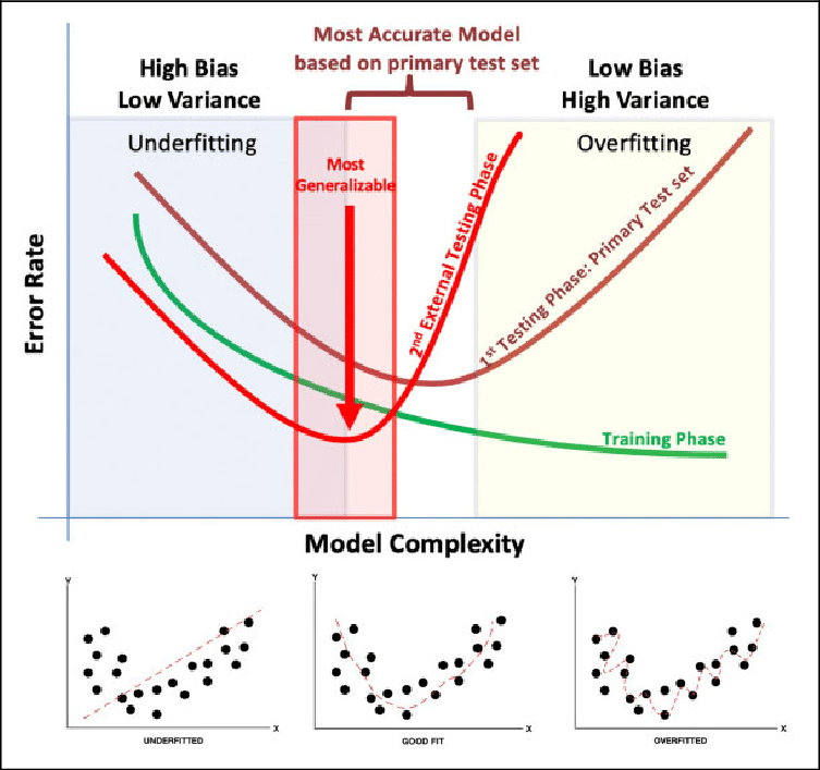
Bias Vs Variance Tradeoff

How do we pick the best model? To address this question, we must first comprehend the trade-off between bias and variance.

The mistake caused by the model’s simple assumptions in fitting the data is referred to as bias. A high bias indicates that the model is unable to capture data patterns, resulting in under-fitting.

The mistake caused by the complicated model trying to match the data is referred to as variance. When a model has a high variance, it passes over the majority of the data points, causing the data to overfit.

From the above program, when degree is 1 which means in linear regression, it shows underfitting which means high bias and low variance. And when we get r2 value 100, which means low bias and high variance, which means overfitting

As the model complexity grows, the bias reduces while the variance increases, and vice versa. A machine learning model should, in theory, have minimal variance and bias. However, having both is nearly impossible. As a result, a trade-off must be made in order to build a strong model that performs well on both train and unseen data.

Degree – how to find the right one?

We need to find the right degree of polynomial parameter, in order to avoid overfitting and underfitting problems,

1. Forward selection: increase the degree parameter till you get the optimal result

2. Backward selection: decrease degree parameter till you get optimal

Loss and Cost function – Polynomial Regression

The Cost Function is a function that evaluates a Machine Learning model’s performance for a given set of data. The Cost Function is a single real number that calculates the difference between anticipated and expected values. Many people are confused by the differences between the Cost Function and the Loss Function. To put it another way, the Cost Function is the average of the n-sample error in the data, whereas the Loss Function is the error for individual data points. To put it another way, the Loss Function refers to a single training example, whereas the Cost Function refers to the complete training set.

The Mean Squared Error may also be used as the Cost Function of Polynomial regression; however, the equation will vary somewhat.

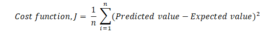
We now know that the Cost Function’s optimum value is 0 or a close approximation to 0. To get an optimal Cost Function, we may use Gradient Descent, which changes the weight and, as a result, reduces mistakes.

Gradient Descent – Polynomial Regression

Gradient descent is a method of determining the values of a function’s parameters (coefficients) in order to minimize a cost function (cost). It may be used to decrease the Cost function (minimizing MSE value) and achieve the best fit line.

The values of slope (m) and slope-intercept (b) will be set to 0 at the start of the function, and the learning rate (α) will be introduced. The learning rate (α) is set to an extremely low number, perhaps between 0.01 and 0.0001. The learning rate is a tuning parameter in an optimization algorithm that sets the step size at each iteration as it moves toward the cost function’s minimum. The partial derivative is then determined in terms of m for the cost function equation, as well as derivatives with regard to the b.

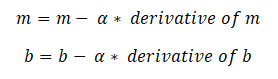
With the aid of the following equation, they and b are updated once the derivatives are determined. m and b’s derivatives are derived above and are α.

Gradient indicates the steepest climb of the loss function, but the steepest fall is the inverse of the gradient, which is why the gradient is subtracted from the weights (m and b). The process of updating the values of m and b continues until the cost function achieves or approaches the ideal value of 0. The current values of m and b will be the best fit line’s optimal value.

Practical application of Polynomial Regression

We will start with importing the libraries,

#with dataset
import numpy as np
import matplotlib.pyplot as plt
import pandas as pd
dataset = pd.read_csv('Position_Salaries.csv')
dataset

Segregating the dataset into dependent and independent features,

X = dataset.iloc[:,1:2].values  
y = dataset.iloc[:,2].values

Then trying with linear regression,

from sklearn.linear_model import LinearRegression
lin_reg = LinearRegression()
lin_reg.fit(X,y)

Visually linear regression can be seen,

plt.scatter(X,y, color='red')
plt.plot(X, lin_reg.predict(X),color='blue')
plt.title("Truth or Bluff(Linear)")
plt.xlabel('Position level')
plt.ylabel('Salary')
plt.show()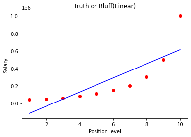

 

from sklearn.preprocessing import PolynomialFeatures
poly_reg = PolynomialFeatures(degree=2)
X_poly = poly_reg.fit_transform(X)

Application of Polynomial Regression

This equation is used to obtain the results in various experimental techniques. The independent and dependent variables have a well-defined connection. It’s used to figure out what isotopes are present in sediments. It’s utilized to look at the spread of various illnesses across a population. It’s utilized to research how synthesis is created.

Advantage of Polynomial Regression

The best approximation of the connection between the dependent and independent variables is a polynomial. It can accommodate a wide range of functions. Polynomial is a type of curve that can accommodate a wide variety of curvatures.

Disadvantages of Polynomial Regression

One or two outliers in the data might have a significant impact on the nonlinear analysis’ outcomes. These are overly reliant on outliers. Furthermore, there are fewer model validation methods for detecting outliers in nonlinear regression than there are for linear regression.

End Notes

Did you find this article to be useful? Please leave your thoughts/opinions in the comments area below. Learning from your mistakes is my favorite quote; if you find something incorrect, simply highlight it; I am eager to learn from readers like you.

About me in short, I am Premanand.S, Assistant Professor Jr and a researcher in Machine Learning. Love to teach and love to learn new things in Data Science. Mail me for any doubt or mistake, [email protected], and my Linkedin https://www.linkedin.com/in/premsanand/