Deep Learning in Medical: Classification of Malaria Infected Blood Cells with ResNet
Photo by Hush Naidoo Jade Photography
Pre-requisite: Basic understanding of Python, Deep Learning, Classification, and Computer Vision
Deep learning is a subset of machine learning and has been applied in various fields to help solve existing problems. One area of application of deep learning is in the medical field. In the medical field, deep learning is beneficial for radiologists. Because the analysis work manually takes a very long time. This article will discuss the classification of malaria-infected blood cells using a deep learning algorithm, Resnet.
This application is publicly accessible online at the following address:
https://www.kaggle.com/muhammadarnaldo/klasifikasi-malaria-cnn/
The dataset used in this article is originated from the official public dataset of the National Institutes of Health (NIH). You can also access this dataset through Kaggle.com.
Importing Library
from keras.optimizers import Adam
from keras.models import Sequential
from keras.layers import Conv2D,MaxPool2D,Flatten,Dense,Dropout,Input,AveragePooling2D
from keras.preprocessing.image import ImageDataGenerator, img_to_array, load_img
from keras.applications import ResNet50V2
from keras.models import Model

%matplotlib inline
from matplotlib import pyplot as plt #untuk visualisasi data
from matplotlib import image as mpimg

from sklearn.metrics import confusion_matrix
import seaborn as sn
import numpy as np #struktur data
The first thing to do is to import the required libraries. The main libraries used in this application are Keras, as the machine learning library; Matplotlib, as the visualization tool; and Sklearn, as the evaluation matrix.
Loading the Dataset
import os
data_dir = "/kaggle/input/cell-images-for-detecting-malaria/cell_images/cell_images"
print(os.listdir(data_dir))
The following is the initial stage, namely importing the required libraries and loading the dataset in the form of images into the environment for processing. Then displays the folder into two categories/classification classes, namely uninfected and parasitized. The libraries used involve Keras and NumPy as deep learning libraries, Sklearn as model evaluation libraries, and Matplotlib to help visualize. Here is the output from the codes above. These two folder names indicate the class name. Uninfected for healthy/normal class, whereas Parasitized is the class for infected patients.
![]()
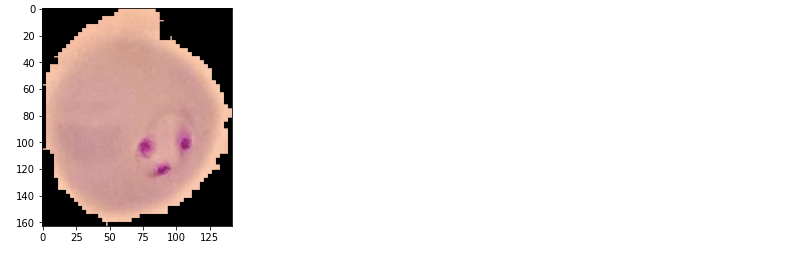
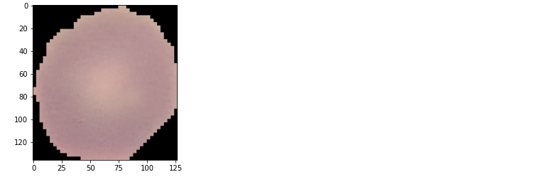
Then we display a preloaded image of infected and healthy cells, to ensure that the data loaded is correct and appropriate. We sample one random image from each class for the display.
img_path="/kaggle/input/cell-images-for-detecting-malaria/cell_images/cell_images/Parasitized/C33P1thinF_IMG_20150619_114756a_cell_179.png"
gambar = mpimg.<a onclick="parent.postMessage({'referent':'.matplotlib.image.imread'}, '*')">imread(img_path)
plt.<a onclick="parent.postMessage({'referent':'.matplotlib.pyplot.imshow'}, '*')">imshow(gambar)
img_path2="/kaggle/input/cell-images-for-detecting-malaria/cell_images/cell_images/Uninfected/C1_thinF_IMG_20150604_104722_cell_60.png"
gambar2 = mpimg.<a onclick="parent.postMessage({'referent':'.matplotlib.image.imread'}, '*')">imread(img_path2)
plt.<a onclick="parent.postMessage({'referent':'.matplotlib.pyplot.imshow'}, '*')">imshow(gambar2)
Preprocessing
dim = 128
batch = 32

datagen =ImageDataGenerator(rescale=1/255.0, validation_split=0.3,
    rotation_range=20,
    zoom_range=0.05,
    width_shift_range=0.05,
    height_shift_range=0.05,
    shear_range=0.05,
    horizontal_flip=True)

train_data =datagen.flow_from_directory(data_dir, target_size=(dim,dim), batch_size=batch, class_mode = 'categorical', subset = 'training')
validation_data =datagen.flow_from_directory(data_dir, target_size=(dim,dim), batch_size=batch, class_mode = 'categorical', subset = 'validation', shuffle=False)
The amount of data used is 27,558, of which 19292 data (70%) are used for training, and 8266 data (30%) are used for testing or validation. In this preprocessing stage, the image is resized to a dimension of 128×128 pixels. Then the grayscale is also applied. In addition, image augmentation is also applied to the dataset. The augmentations used are rotation, zoom, width shift, height shift, shear, and flip horizontally.
Create the Model
baseModel =ResNet50V2(include_top=False,
                     input_tensor=Input(shape=(dim,dim, 3)))

headModel =baseModel.outputheadModel =AveragePooling2D(pool_size=(4, 4))(headModel)
headModel =Flatten(name="flatten")(headModel)
headModel =Dense(128, activation="relu")(headModel)
headModel =Dropout(0.5)(headModel)
headModel =Dense(2, activation="softmax")(headModel)

model =Model(inputs=baseModel.input, outputs=headModel)

model.summary()
At this stage, the model is formed. Base CNN architecture using ResNet-50. As the name suggests, the model developed has 50 convolution layers along with their pooling layers. At the end of the model, there are two fully connected layers. The first layer consists of 128 neurons with ReLU activation. The second layer consists of 2 neurons representing the number of classification classes, using softmax activation. Between these fully connected layers, there is a dropout layer, and the configuration is set to 50%. The total parameters/weights in this model are 23,827,330. This model uses transfer learning from the pre-trained model on the ImageNet dataset. But the coding is not shown (implicit). This transfer learning process is used to speed up the training process. The input image goes to convolution and pooling. This convolution and pooling layer will be repeated. Between layers, there is also batch normalization for regulation and there is an activation layer. In the ResNet model, there is a layer that is quite important, namely the additional layer. That is the sum of the residues from the previous convolution layer on the next convolution layer. This is the hallmark of ResNet which is also a revolution in the world of deep learning.
Training Process
The configurations for the training process are as follows:
EP = 30

model.compile(optimizer="adam",
              loss="binary_crossentropy",
              metrics=["accuracy"])

history =model.fit(train_data, validation_data=validation_data, epochs=EP)
print("*** proses training selesai ***")
The training process is carried out with 30 epochs, with Adam optimizer. The loss function used is the binary cross-entropy, because we only have two classes to classify. The model.fit will run the training process. The training process includes validation data in order to track overfitting in the evaluation step.
Evaluation
plt.style.use("ggplot")
plt.figure()

plt.plot(np.arange(0,EP),history.history["loss"], label="train_loss")
plt.plot(np.arange(0,EP),history.history["val_loss"], label="val_loss")
plt.plot(np.arange(0,EP),history.history["accuracy"], label="train_acc")
plt.plot(np.arange(0,EP),history.history["val_accuracy"], label="val_acc")

plt.title("Training Loss and Accuracy")
plt.xlabel("Epoch #")
plt.ylabel("Loss/Accuracy")
plt.legend(loc="lower left")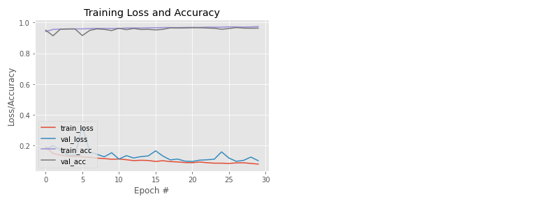
test_loss, test_acc = model.evaluate(validation_data)

The accuracy results obtained are 96.19% of the testing data. In the previous plot, it can be seen that the training and testing lines are close together and do not show any overfitting.
Two purple lines that are at the top of the graph indicate accuracy, and the accuracy looks relatively stable and increasing. In comparison, the red and blue lines at the bottom of the chart indicate the loss.
Classification Evaluation with Confusion Matrix
predictions = model.predict(validation_data)
y_pred =np.argmax(predictions, axis=-1)
#y_pred = [1 * (x[0]>=0.5) for x in predictions]cf_matrix =confusion_matrix(validation_data.classes,y_pred)
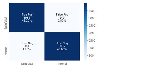
group_names = ["True Pos","False Pos","False Neg","True Neg"]
group_counts = ["{0:0.0f}".format(value) forvalueincf_matrix.flatten()]
group_percentages = ["{0:.2%}".format(value) forvalueincf_matrix.flatten()/np.sum(cf_matrix)]
labels = [f"{v1}\n{v2}\n{v3}" forv1,v2,v3inzip(group_names,group_counts,group_percentages)]
labels =np.asarray(labels).reshape(2,2)
categories = ["Terinfeksi","Normal"]
sn.heatmap(cf_matrix, annot=labels, fmt='', xticklabels=categories, yticklabels=categories, cmap='Blues')
The following confusion matrix shows that the model is able to generalize well. Whether it’s for the classification of infected images as well as the classification of normal images. Sensitivity and Specificity are evenly distributed.
Wrong predictions on infected and normal images also appear to be at the threshold of only 2%. So We can conclude that the use of ResNet-50 in malaria image classification got good results.
Saving the Model
We can save the model in Hierarchical Data Format h5 format with the following code for later use.
model.save('./cnn_malaria_binary.h5')
Conclusion
- Deep learning can be implemented in the medical field, especially in malaria classification;
- Resnet-50 has proven to be able to generalized well in medical image classification;
- The deep learning architecture with the above configuration successfully achieved good accuracy 96,19% without overfitting.
What’s next
- Build a deep learning implementation in another field;
- Create a classification using the current dataset with another deep learning algorithm.
Author Bio
My name is Muhammad Arnaldo, a machine learning and data science enthusiast. Currently pursuing the master of computer science in Indonesia.
The media shown in this article is not owned by Analytics Vidhya and are used at the Author’s discretion.


