How a Math equation is used in building a Linear Regression model?
This article was published as a part of the Data Science Blogathon
Table of Contents
- Overview
- What is Regression?
- Independent Variables
- Dependent Variables
- Linear Regression
- The Equation of a Linear Regression
- Types of Linear Regression
- Simple Linear Regression
- Multiple Linear Regression
- How is a simple linear equation used in the ML Linear Regression algorithm?
- Drop the unnecessary feature column in the given data set
- How to Know the size of the given data set?
- How to get Complete information of the given data set?
- Check the number of missing values in the given data set
- How to visualize the data that has got linear relation between the feature and target column?
- Separate the feature and target column
- How to use SK learn Linear Regression for a data set?
- How to find model Coefficients for linear regression model in SK learn?
- Conclusion
Overview
Let us see a simple and very easy way of building a simple linear regression model.
- If you are very new to data science or artificial intelligence or the machine learning field
- If you are a beginner and want to know what an ML model is
- If you want to build a simple ML model with the mathematical equation which we have studied in our high school and colleges, etc.
What is Regression?
The font size of the below section looks smaller – Pls check, can’t fix it from here
In Statistical terms, regression is a measure of the relation between the mean of one variable with the other variable. For example time and cost.
Let us try to understand in normal terms, regression is an attempt to determine the relationship between one dependent and a series of other independent variables. I hope you got an idea of what regression is all about.
Independent Variables
These independent variables in Machine Learning are termed by different names like:
- Feature columns or variables
- Input columns or variables
Dependent Variables
And the dependent variables in Machine Learning are termed by different names like:
- Label column or variable
- Output column or variable
Linear Regression
Linear Regression is a machine learning algorithm where we find the relationship between the feature and the target columns. We always look for a Linear relationship, that is if a simple straight line can be drawn between the features and target column then we decide to go and build a linear model.
Let us get much deeper now. From the school days, we have come across the equation of the straight line i.e. y = mx + c, right? Haven’t we? Yes, we have in fact, a lot many times. Do you know that this one equation helps in building a linear regression model in the machine learning world? Yes, you heard it right. The entire Linear regression is built on this equation.
Linear Regression is one of the most fundamental and widely known ML algorithms which people start with. Building blocks of a Linear Regression Model are:
- The independent variables must be Discrete/continuous
- The dependent variable must be Continuous.
- A best-fit regression line
The Equation for a Linear Regression
A Linear equation is given by:
Y = m X + b + e
Where b is the intercept, m is the slope of the line, and e is the error term. The equation above is used to predict the value of the target variable based on the given predictor variable(s).
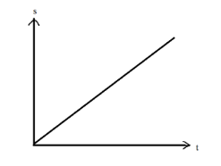
A linear relationship typically looks like this:
Types of Linear Regression
There are two types of linear regression model we can build based on the number of feature columns present in the data set:
- Simple Linear Regression
-
Multiple Linear Regression
Simple Linear Regression
If the data set contains only 1 feature and 1 target column then that is called simple Linear Regression.
The equation of a simple linear regression is given by:
Y = m X + b
Y – Target or Output
X – Feature column
m and b are model coefficients. The values of m and b are found by using the machine learning linear regression model. So for a given input value, the ML model predicts the output based on the values of m and b.
We have the below data set with 1 feature and 1 target column,
| X
|
Y |
| 1 | 10 |
| 2 | 20 |
| 3 | 50 |
| 4 | 40 |
| 5 | 20 |
Say for example if m=10, c=1, and x is 6 so the model needs to predict their value. So using the equation we can get y=(10*6) + 1 then the Y value is 61 for the given input.
Multiple Linear Regression
| X1 | X2 | X3 | Y |
| 1 | 0 | 0 | 0 |
| 0 | 0 | 0 | 1 |
| 0 | 1 | 1 | 0 |
| 1 | 0 | 1 | 0 |
| 1 | 1 | 1 | 1 |
Say for example given x1=0, x2=1, x3=0 input values the model predicts the coefficients (m1=1, m2=0,m3=1) and intercept as is 0. What’s the value of y?. So using the above equation we can get y=(1*0)+(0*1)+(1*0) + 0 then Y value is 0 for given inputs.
Now let us get deeper into linear model prediction.
How is a simple linear equation used in Machine Learning Linear Regression Algorithm?
Now, let’s take an example with a simple machine learning data set.
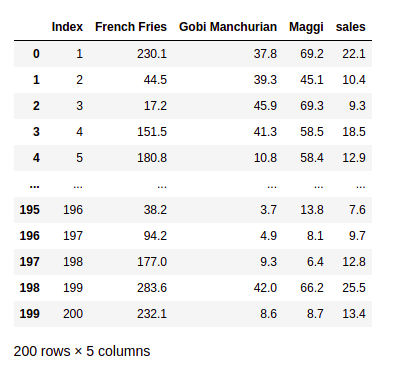
The above data set is data of a hotel where it describes the sales made for each food recipe at different costs. The numbers taken are at random to build a linear regression model, where the amount of price cost doesn’t represent the present market price in Indian rupees.
Let’s explore what we have learned above with the data set and the linear equation. Here in the given hotel data set the feature columns are :
- French Fries
- Gobi Manchurian
- Maggi
And the target column is
- Sales
So now once the data set is given we must do exploratory data analysis like checking for missing values, treating the left or right skewness, replacing the special symbols, etc.
We check for the normal distribution for the given data set. Suppose if the data set is not normally distributed then we do the standard scaling and normalization for any given data set before building a machine learning model as it leads to better accuracy and model score.
Drop unnecessary feature column in the given dataset
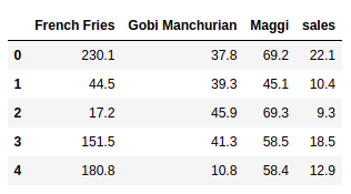
In the given hotel data set, the column Index does not involve any decision-making. Where the model doesn’t learn any pattern. So let’s drop this column using pandas data frame,
data.drop(['Index'], axis=1,inplace=True)
And now let us see the data set by selecting only the first 5 rows,
How to Know the Size of the given data set?
data.shape
In the given data set there are 200 rows and 4 columns( as we have deleted one).
How to get Complete information of the given data set?
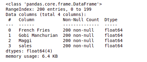
Use data frame info method to get the entire data set information with the column names and their data types and with non-nulls values,
data.info()
Check the number of missing values in the given data set
Now let us get into the actual data analysis part, where we must treat the missing values by replacing them with mean or mode.
data.isna().sum()
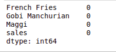
Here in the above data set, there are no null or missing values. So we are good to go and apply the simple linear regression. In real-time we do a lot of analysis on the data and perform feature engineering, feature selection, and EDA operation before applying any of the ML algorithms.
How to visualize the data that has got linear relation between the feature and target column?
fig, axs = plt.subplots(1, 3, sharey=True)
data.plot(kind='scatter', x='French Fries', y='sales', ax=axs[0], figsize=(16, 8))
data.plot(kind='scatter', x='Gobi Manchurian', y='sales', ax=axs[1])
data.plot(kind='scatter', x='Maggi', y='sales', ax=axs[2])
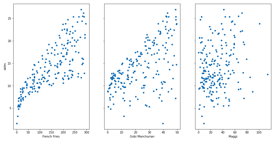
Here we see that there is a linear relationship between some of the features and the target column. A generic question to be asked?
- What’s the relationship between features and target?
- How prominent is that relationship?
- How does each feature column contribute to the target?
Let us explore the above questions.
From the diagrams above, it can be observed that there seems to be a linear relationship between the features of French Fries and sales. And similarly Gobi Manchurian and the sales are almost a linear one.
So the basic prerequisite for applying the simple linear regression holds good, so now let’s apply the machine learning linear regression algorithm to the hotel data set.
Separate the Feature and Label Column
We need to separate the features columns and the label column as the X and Y variables. So we can pass this for model prediction,
feature_cols = ['French Fries', 'Gobi Manchurian', 'Maggi']
X = data[feature_cols]
Y = data.sales
How to use SKLearn Linear Regression for a data set?
We are importing the linear regression from the Scikit Learn library,
from sklearn.linear_model import LinearRegression
we instantiate the Linear regression and apply a direct model. fit() on the feature and target columns
slr = LinearRegression()
slr.fit(X, Y)
How to find model coefficients for the Linear regression model in sklearn?
Once the model is trained we check for values of m and c for a simple linear equation of line y = mx + c.
print('c value is: ',slr.intercept_)
print('m1, m2 and m3 values are: ',slr.coef_)

Conclusion
I restrict my article here as it was more focused on how a simple linear equation in math is used in Machine Learning algorithms and using which we build an ML model for predicting the target values.
I hope you enjoyed this article. And you could relate the math equation with that of a Machine Learning algorithm.
Thanks for Reading
The media shown in this article is not owned by Analytics Vidhya and are used at the Author’s discretion.


