Logistic Regression: An Introductory Note
This article was published as a part of the Data Science Blogathon.
Introduction
Linear regression maps a vector x to a scalar y. If we can squash the Linear regression output in the range 0 to 1, it can be interpreted as a probability. We can have a classifier that gives the class label’s probability for binary classification tasks by squashing a linear regression model output. This supervised learning classifier is known as a Logistic regression classifier.
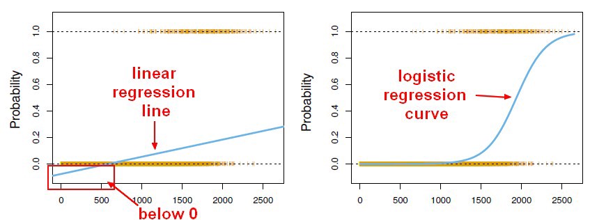
Here, the sigmoid function, also known as the logistic function, predicts the likelihood of a binary outcome occurring. The Sigmoid Function is an activation function used to introduce non-linearity to a machine learning model. It takes a value and converts it between 0 and 1. The function is as follows:

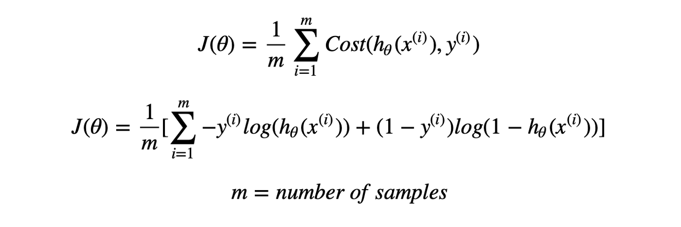
Thus, Logistic regression predicts the class label by identifying the connection between the independent feature variables. The decision boundary is linear, which is used for classification purposes. The loss function is as follows:
Advantages of Logistic Regression
- The logistic regression model is easy to implement.
- It is very efficient to train.
- It is less prone to overfitting.
- This classifier performs efficiently with the linearly separable dataset.
Disadvantages of Logistic Regression
- This model is used to predict only discrete functions.
- The non-linear problems cannot be solved using a logistic regression classifier.
Applications
- Classifying whether an email is spam or not
- Classifying the quality of water is good or not
Dataset
The Dataset used for this project is the Wine Quality Binary classification dataset from Kaggle (https://www.kaggle.com/nareshbhat/wine-quality-binary-classification). This Data set contains information related to the various factors affecting the quality of red wine.
Number of Instances: 1600
Missing values: NA
Number of Attributes: 12
Attribute Information:
Input variables: (all numeric valued)
1 – fixed acidity
2 – volatile acidity
3 – citric acid
4 – residual sugar
5 – chlorides
6 – free sulfur dioxide
7 – total sulfur dioxide
8 – density
9 – pH
10 – sulphates
11 – alcohol
Output variable : (detect whether the quality is good or bad)
12 – quality (0-bad, 1-good)
Import the required Python libraries
import pandas as pd
import numpy as np
import matplotlib.pyplot as plt
import seaborn as sns
import warnings
warnings.filterwarnings('ignore')
Load the dataset
We will load our wine dataset, a CSV file using the panda’s library of Python.
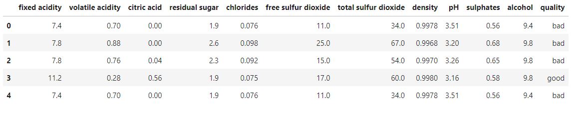
df=pd.read_csv("wine.csv")
df.head()
Data Preprocessing
#preprocessing
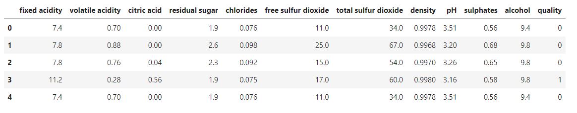
#The quality column in the dataset has to be mapped as- 0 for bad and 1 for good.
df = df.replace({'quality': {'good': 1, 'bad': 0}})
df.head()
Check for missing values
#checking for missing values
df.isna().any().any()
Output: False
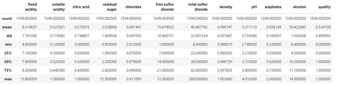
Overall statistics and plots
df.describe()
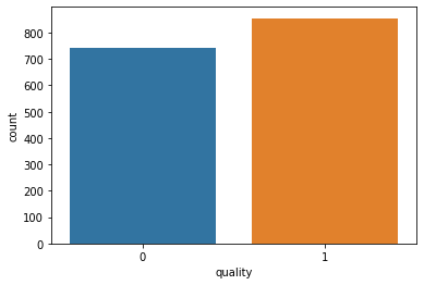
#We will use a countplot to visualize the count of observations for ‘quality’ column.
sns.countplot(x ='quality', data = df)
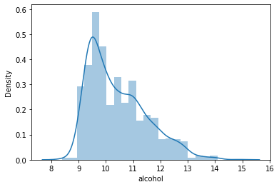
#Distribution of the column – alcohol
data = df['alcohol']
sns.distplot(data)
plt.show()
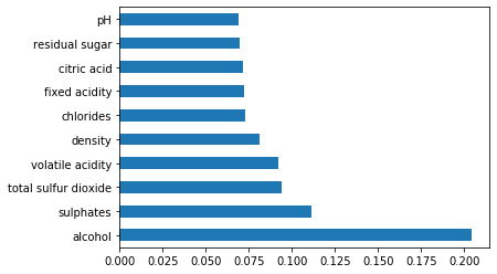
Feature Importance Score
import warnings
warnings.filterwarnings('ignore')
from sklearn.ensemble import ExtraTreesClassifier
model = ExtraTreesClassifier()
model.fit(features,target)
print(model.feature_importances_)
imp = pd.Series(model.feature_importances_, index=features.columns)
imp.nlargest(10).plot(kind='barh')
plt.show()
Defining Features and the Target Variable
#features used for classification include –
#alcohol, sulphates, total sulphur dioxide, volatile acidity, citric acid and residual sugar.
#target=quality
target = df.iloc[:,11]
features=df.iloc[:,[10,9,6,1,2,3]]
Standardize the Feature Vectors
#standardize feature vectors
from sklearn.preprocessing import StandardScaler
#StandardScaler() will rescale the feature values so that their standard deviation is 1 and .mean is 0.
sc=StandardScaler()
scaled_features=sc.fit_transform(features)
Logistic Regression Model
We will be using the logistic regression inbuilt model from the sklearn library of Python, where we can also define the loss function and make the predictions.
We will start by first splitting our dataset into two parts; one as a training set for the model and the other as a test set to validate the model’s predictions. If we omit this step, the model will be trained and tested on the same dataset, and it’ll underestimate the true error rate, a phenomenon called overfitting. We will set the test size to 0.3, i.e., 70% of the class label will be assigned to the training set, and the remaining 30% will be used as a test set. We will do this using the train_test_split method in the sklearn library of Python. The model. fit() method can take the training data as arguments. Here our model name is LR. This model takes some unlabeled data from the test dataset and can effectively assign each example a probability ranging from 0 to 1. This is the crucial feature of a Logistic regression model. Then we will be evaluating our model on the test data.
Logistic regression using Standard Gradient Descent algorithm with split 70:30
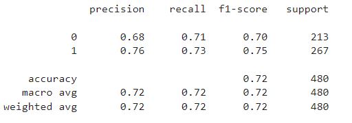
from sklearn.linear_model import LogisticRegression
from sklearn.linear_model import SGDClassifier
#70% training data
X_train, X_test, y_train, y_test = train_test_split(scaled_features, target, test_size=0.3, random_state=42)
lr=LogisticRegression()
lr.fit(X_train,y_train)
print(classification_report(y_test,lr.predict(X_test)))
Logistic regression using Gradient Descent from Scratch
The cost function of a Logistic regression model can be minimized by using Gradient descent as follows:
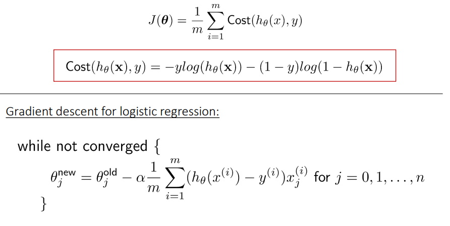
It is an iterative optimization algorithm and finds the minimum of a differentiable function. First, you need to select any random point from the function. Then it would help if you computed the derivative of the function. Now you can multiply the resultant gradient with our learning rate. Then you need to subtract the result to get the new. This update should be simultaneously done for every iteration. Repeat these steps until you reach the local or global minimum. You have achieved the lowest possible loss in your prediction by reaching the global minimum.
from sklearn.datasets.samples_generator import make_blobs
from matplotlib import pyplot as plt
from pandas import DataFrame
import numpy as np
X, Y = make_blobs(n_samples=100, centers=2, n_features=2, cluster_std=5, random_state=11)
m = 100
#returns an array containing sigmoid of the input array
def sigmoid(z):
    return 1 / (1 + np.exp(-z))

#returns an array containing the predictions of our input array
def hy(w,X):
    z = np.array(w[0] + w[1]*np.array(X[:,0]) + w[2]*np.array(X[:,1]))
    return sigmoid(z)

#cost function
def cost(w, X, Y):
    y_predictions = hy(w,X)   #assigning the prediction values
    return -1 * sum(Y*np.log(y_predictions) + (1-Y)*np.log(1-y_predictions))
#gradient descent
def partial_derivatives(w, X, Y):
    y_predictions = hy(w,X)
    j = [0]*3
    j[0] = -1 * sum(Y*(1-y_predictions) - (1-Y)*y_predictions)   #storing partial derivatives
    j[1] = -1 * sum(Y*(1-y_predictions)*X[:,0] - (1-Y)*y_predictions*X[:,0])
    j[2] = -1 * sum(Y*(1-y_predictions)*X[:,1] - (1-Y)*y_predictions*X[:,1])
    return j  #returns array containg partial derivatives

def gradient_descent(w_new, w_prev, learning_rate):
    print(w_prev)
    print(cost(w_prev, X, Y))
    j=0
    while True:
        w_prev = w_new    #updating weights in each iteration
        w0 = w_prev[0] - learning_rate*partial_derivatives(w_prev, X, Y)[0]
        w1 = w_prev[1] - learning_rate*partial_derivatives(w_prev, X, Y)[1]
        w2 = w_prev[2] - learning_rate*partial_derivatives(w_prev, X, Y)[2]
        w_new = [w0, w1, w2]
        print(w_new)
        print(cost(w_new, X, Y))
        if (w_new[0]-w_prev[0])**2 + (w_new[1]-w_prev[1])**2 + (w_new[2]-w_prev[2])**2 100:
            return w_new
        j+=1
w=[1,1,1]
w = gradient_descent(w,w,0.0099)
print(w)
def equation(x):
return (-w[0]-w[1]*x)/w[2]
def graph(formula, x_range):
x = np.array(x_range)
y = formula(x)
plt.plot(x, y)
df = DataFrame(dict(x=X[:,0], y=X[:,1], label=Y))
colors = {0:'red', 1:'green'}
fig, ax = plt.subplots()
g = df.groupby('label')
for key, group in g:
group.plot(ax=ax, kind='scatter', x='x', y='y', label=key, color=colors[key])
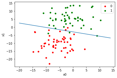
graph(equation, range(-20,15))
plt.xlabel('x0')
plt.ylabel('x1')
plt.show()
Read more articles based on Logistic Regression on our website.
Conclusion
Thus, Logistic regression is a statistical analysis method. Our model has accurately labeled 72% of the test data, and we could increase the accuracy even higher by using a different algorithm for the dataset.
The media shown in this article is not owned by Analytics Vidhya and are used at the Author’s discretion.


