Approaching Regression with Neural Networks Using Tensorflow

This article was published as a part of the Data Science Blogathon.

Introduction

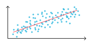
Every supervised machine learning technique basically solves either classification or regression problems. Classification is a kind of technique where we classify the outcome into distinct categories whose range is usually finite. Whereas a regression technique involves predicting a real number whose range is infinite. Some examples of regression are predicting the price of a house given the number of bedrooms and floors in it or predicting the product rating given specifications of the product etc.

Neural networks are one of the most important algorithms that have profound applications in computer vision and natural language processing domains. Now let’s apply these neural networks on tabular data for a regression task. We will use Tensorflow and Keras deep learning library to build and train our neural network.

Let’s get started…

About the Dataset

The dataset we are using to train our model is the Auto MPG dataset. This dataset consists of different features of commonly used automobiles during the 1980s and 90s. This includes attributes like the number of cylinders, horsepower, the weight of the car etc. Using these features we should predict the miles per gallon or mileage of the automobile. Thus making it a multi-variate regression task. More information about the dataset can be found here.

Getting Started

Let’s get started by importing the required libraries and downloading the dataset.

import pandas as pd
import matplotlib.pyplot as plt
import tensorflow as tf
from tensorflow import keras
from tensorflow.keras import layers
from tensorflow.keras import Sequential
from tensorflow.keras import optimizers

Now let’s download and parse the dataset using pandas into a data frame.

url = "http://archive.ics.uci.edu/ml/machine-learning-databases/auto-mpg/auto-mpg.data"
column_names = ["MPG", "Cylinders", "Displacement", "Horsepower", "Weight",
                "Acceleration", "Model Year", "Origin"]
df = pd.read_csv(url, names=column_names, sep=" ",
                 comment="t", na_values="?", skipinitialspace=True)

We have directly downloaded the dataset using the pandas read_csv method and parsed it to a data frame. We can check the contents of the data frame for more details.

df.head()

Now let’s preprocess this data frame to make it easier for our deep learning model to understand. Before that, it is a good practice to make a copy of the original dataset and then work on it.

# Create a copy for further processing
dataset = df.copy()
# Get some basic data about dataset
print(len(dataset))

Data Preprocessing

Now let’s preprocess our dataset. First, let’s check for null values since it is important to handle all null values before feeding the data into our model (If data consists of null values, the model won’t be able to learn resulting in null results).

# Check for null values
dataset.isna().sum()

Since we encountered some null values in the ‘Horsepower’ column, we can handle them easily using the Pandas library. We can usually drop all the null values using dropna() method or also fill those null values with some value like the mean of the entire column etc. Let’s use fillna() method to fill the null values.

# There are some na values. We can fill or remove those rows.
dataset['Horsepower'].fillna(dataset['Horsepower'].mean(), inplace=True)
dataset.isna().sum()

Now we can see that there are no null values present in any columns. According to the dataset, the ‘Origin’ column is not numeric but categorical i.e. each number represents each country. So let’s encode this column by using the pandas get_dummies() method.

dataset['Origin'].value_counts()
dataset['Origin'] = dataset['Origin'].map({1: 'USA', 2: 'Europe', 3: 'Japan'})
dataset = pd.get_dummies(dataset, columns=['Origin'], prefix='', prefix_sep='')
dataset.head()

For the above output, we can observe that the single ‘Origin’ column is replaced by 3 columns with the names of the countries with 1 or 0 representing the origin country.

Now, let’s split the dataset into training and testing/validation set. This is useful to test the effectiveness of the model i.e. how good the model generalises on the unseen data.

# Split the Dataset and create train and test sets
train_dataset = dataset.sample(frac=0.8, random_state=0)
test_dataset = dataset.drop(train_dataset.index)
########################################################
# Separate labels and features
train_features = train_dataset.drop(["MPG"], axis=1)
test_features = test_dataset.drop(["MPG"], axis=1)
train_labels = train_dataset["MPG"]
test_labels = test_dataset["MPG"]

We can check some basic statistics about the data using the pandas describe() function.

# Let's check some basic data about dataset
train_dataset.describe().transpose()

We can now proceed with the next data preprocessing step: Normalization.

Data normalization is one of the basic preprocessing steps which will convert the data into a format that the model can easily process. In this step, we scale the data such that the mean will be 0 and the standard deviation will be 1. We will use the sci-kit learn library to do the same.

# But we can also apply normalization using sklearn.
from sklearn.preprocessing import StandardScaler
feature_scaler = StandardScaler()
label_scaler = StandardScaler()
########################################################
# Fit on Training Data
feature_scaler.fit(train_features.values)
label_scaler.fit(train_labels.values.reshape(-1, 1))
########################################################
# Transform both training and testing data
train_features = feature_scaler.transform(train_features.values)
test_features = feature_scaler.transform(test_features.values)
train_labels = label_scaler.transform(train_labels.values.reshape(-1, 1))
test_labels = label_scaler.transform(test_labels.values.reshape(-1, 1))

We do the fit and transform separately because the fit will learn the data representation of the input data and transform will apply the learnt representation. In this way, we will be able to avoid looking at the representation/statistics of the test data.

Now let’s get into the most exciting part of the process: Building our neural network.

Creating the Model

Let’s create our model by using the Keras Sequential API. We can stack the required layers into the sequential model and then define the required architecture. Now let’s create a basic fully connected dense neural network for our data.

# Now let's create a Deep Neural Network to train a regression model on our data.
model = Sequential([
    layers.Dense(32, activation='relu'),
    layers.Dense(64, activation='relu'),
    layers.Dense(1)
])

We have defined the sequential model by adding 2 dense layers with 32 and 64 units respectively, both using the Rectified Linear Unit activation function i.e. Relu. Finally, we are adding a dense layer with 1 neuron representing the output dimension i.e. a single number. Now let’s compile the model by specifying the loss function and optimizer.

model.compile(optimizer="RMSProp",
              loss="mean_squared_error")

For our model, we are using the RMSProp optimizer and the mean squared error loss function. These are important parameters for our model because the optimizer defines how our model will be improved and loss defines what will be improved.

It is recommended to try updating/playing with the above model by using different layers or changing the optimizers and loss function and observing how the model performance improves or worsens.

Now we are ready to train the model !!

Model Training and Evaluation

Now let’s train our model by specifying the training features and labels for 100 epochs. We can also pass the validation data to periodically check how our model is performing.

# Now let's train the model
history = model.fit(epochs=100, x=train_features, y=train_labels,
          validation_data=(test_features, test_labels), verbose=0)

Since we specified the verbose=0, we won’t get any model training log for every epoch. We can use the model history to plot how our model has performed during the training. Let’s define a function for the same.

# Function to plot loss
def plot_loss(history):
    plt.plot(history.history['loss'], label='loss')
    plt.plot(history.history['val_loss'], label='val_loss')
    plt.ylim([0,10])
    plt.xlabel('Epoch')
    plt.ylabel('Error (Loss)')
    plt.legend()
    plt.grid(True)
########################################################
plot_loss(history)

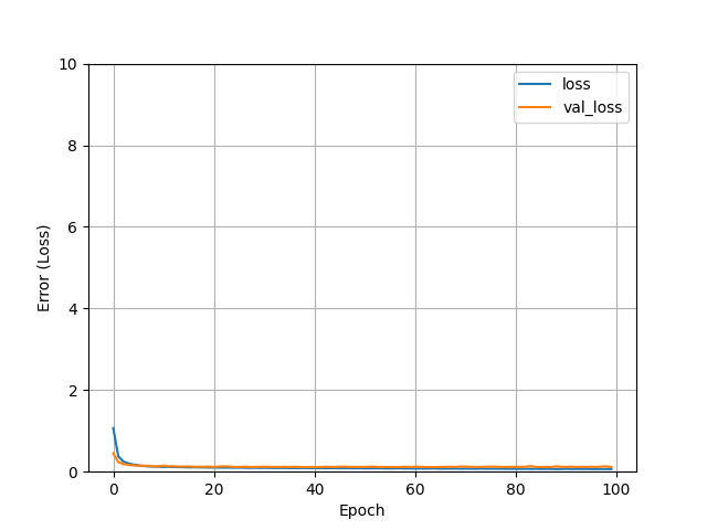
Now we can see that our model has been able to achieve the least loss during the training. This is due to the fully connected layers through which our model was able to easily detect the patterns in the dataset.

Now finally let’s evaluate the model on our testing dataset.

# Model evaluation on testing dataset
model.evaluate(test_features, test_labels)

The model performed well on the testing dataset! We can save this model and use the saved model to predict some other data.

# Save model
model.save("trained_model.h5")

Now, we can load the model and perform predictions.

# Load and perform predictions
saved_model = models.load_model('trained_model.h5')
results = saved_model.predict(test_features)
########################################################
# We can decode using the scikit-learn object to get the result
decoded_result = label_scaler.inverse_transform(results.reshape(-1,1))
print(decoded_result)

Oh great !! Now we can see the predictions i.e. decoded data given the input features into our model.

Conclusion

In the blog on regression with neural networks, we have trained the baseline regression model using deep neural networks on a small and simple dataset and predicted the required output. As a challenge for learning, it is recommended to train more models on bigger datasets by changing the architecture and trying different hyperparameters such as optimizers and loss functions. Hope you liked my article on regression with neural networks.

References

Image 1: https://www.tibco.com/reference-center/what-is-regression-analysis

About the Author

I’m Narasimha Karthik, Deep Learning Practioner. I’m a final-year undergraduate student at PES University. Currently working with Computer Vision and NLP. Experience in working with Tensorflow and PyTorch frameworks. You can contact me through LinkedIn and Twitter.

Read more articles on our blog.

The media shown in this article is not owned by Analytics Vidhya and are used at the Author’s discretion.