A Basic Introduction to Activation Function in Deep Learning
This article was published as a part of the Data Science Blogathon.
Introduction
The activation function is defined as follows: The activation function calculates a weighted total and then adds bias to it to decide whether a neuron should be activated or not. The Activation Function’s goal is to introduce non-linearity into a neuron’s output.
A Neural Network without an activation function is basically a linear regression model in Deep Learning, since these functions perform non-linear computations on the input of a Neural Network, enabling it to learn and do more complex tasks. Therefore, studying the derivatives and application of activation functions, also as analysing the pros and drawbacks of each activation function, is essential for selecting the proper type of activation function that may give non-linearity and accuracy in a particular Neural Network model.
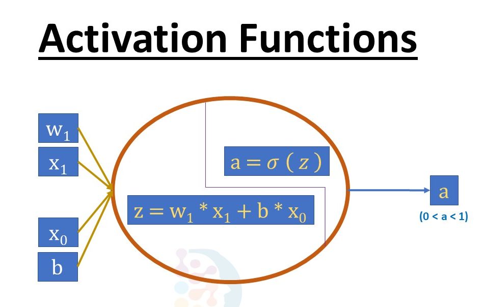
We know that neurons in a Neural Network work following their weight, bias, and activation function. We would change the weights and biases of the neurons in a Neural Network based on the output error. Back-propagation is the term for this process. Because the gradients are supplied simultaneously with the error to update the weights and biases, activation functions, therefore, enable back-propagation.
Table of Contents
- Why Do We Need Activation Functions in CNN?
- Variants Of Activation Function
- Python Code Implementation
- Conclusion
Why do we need it?
Non-linear activation functions: Without an activation function, a Neural Network is just a linear regression model. The activation function transforms the input in a non-linear way, allowing it to learn and as well as accomplish more complex tasks.
Mathematical proof:-
The diagram’s elements include:- A hidden layer, i.e. layer 1:- A visible layer, i.e. layer 2:- A visible layer, i.e.
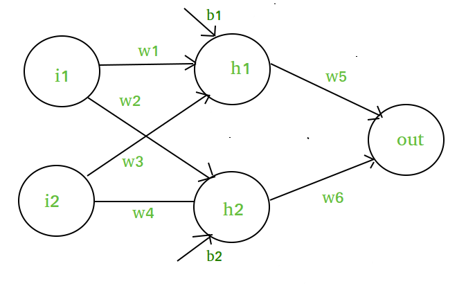
Source: geeksforgeeks.com
a(1) = z(1)
= W(1)X + b(1) (1)
Here,
Layer 1’s vectorized output is z(1).
W(1) denotes the vectorized weights (w1, w2, w3, and w4) applied to hidden layer neurons, X denotes the vectorized input features (i1 and i2), and b denotes the vectorized bias (b1 and b2).
Any linear function has a(1) being vectorized form.
(Note that the activation function is not taken into consideration here.)
The output layer, or layer 2, is as follows:
Layer 2 input is z(2) = W(2)a(1) + b(2) a(2) = z(2)a(1) + b(2) a(2) = z(2)a(1) + b(2) a(2) = z(2)a(1) + b(2) a(2) = z(2)a(1) + b(2) a(2) (2)
Output layer calculation:
/ Here’s where we’ll put the value of z(1).
(W(2) * [W(1)X + b(1)]) + b = (W(2) * [W(1)X + b(1)]) (2)
[W(2) * W(1)] = z(2) * [W(2)*b(1) + b(2)] + XLet,
W = [W(2) * W(1)]
b = [W(2)*b(1) + b(2)]
z(2) = W*X + b is the final result.
Which is a linear function once again.
Even after applying a hidden layer, this observation yields a linear function, hence we can deduce that no matter how many hidden layers we add to a Neural Network, all layers will behave the same way because the combination of two linear functions yields a linear function.
Variants Of Activation Function
1). Linear Function: –
• Equation: The equation for a linear function is y = ax, which is very much similar to the equation for a straight line.
• -inf to +inf range
• Applications: The linear activation function is only used once, in the output layer.
.jpg)
• Problems: If we differentiate a linear function to introduce non-linearity, the outcome will no longer be related to the input “x” and the function will become constant, hence our procedure will not show any behaviour.
For example, determining the price of a home is a regression problem. Because the price of an apartment might be a large or little number, we can employ linear activation at the output layer. Even in this case, any non-linear function at the hidden layers of the Neural Network is required.
2) The sigmoid function:
• It’s a function that is being plotted in the form of ‘S’ Shape.
• Formula: A = 1/(1 + e-x)
• Non-linear in nature. The values of X ranges from -2 to 2, but the Y values are highly steep. This indicates that slight changes in x will result in massive changes in Y’s value.
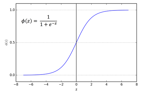
• 0 to 1 value of the range
3). Tanh Function: Tanh function, also identified as Tangent Hyperbolic function, is an activation that almost always works better than sigmoid function. It’s simply a sigmoid function that has been adjusted. Both are related and can be deduced from one another.
• Equation: f(x) = tanh(x) = 2/(1 + e-2x) – 1 OR tanh(x) = 2 * sigmoid(2x) – 1 OR tanh(x) = 2 * sigmoid(2x) – 1
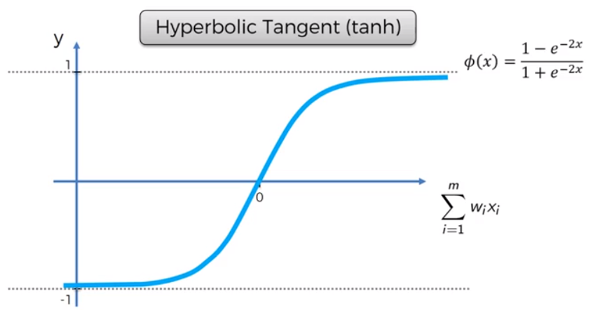
• Range of values: -1 to +1
• Uses:- Usually employed in hidden layers of a Neural Network since its values change from -1 to 1, causing the hidden layer’s mean to be 0 or very close to it, which aids in data centring by bringing the mean close to 0. This makes learning the next layer much more straight.
4). RELU (Rectified linear unit) is the fourth letter in the alphabet. It’s the most used activation method. Hidden layers of neural networks are primarily used.
• Formula: A(x) = maximum (0,x). If x is positive, it returns x; else, it returns 0.
• Value Range: (inf, 0)
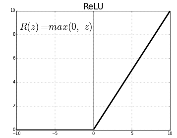
Source: Medium.com
• Non-linear in nature, which means simply backpropagating errors and also having the ReLU function activating many layers of neurons.
• Applications: Because it includes fewer mathematical operations, ReLu is less computationally expensive than tanh and sigmoid. Only a few neurons are active at a time, making the network scarce and efficient for computation.
Simply put, the RELU function learns much faster than the sigmoid and Tanh functions.
5). Softmax Function: The softmax function is a type of sigmoid function that comes in handy when dealing with categorization issues.
• Non-linearity in nature
• Uses: Typically utilised when dealing with many classes. The softmax function would divide by the sum of the outputs and squeeze the outputs for each class between 0 and 1.

• Output: The softmax function is best used in the classifier’s output layer, where we’re trying to define the class of each input using probabilities.
Selecting The Right Activation Function
If one is unsure about the activation function to utilise, just select RELU, which is a broad activation function that is used in most circumstances these days. If our output layer is meant to be used for binary identification/detection, the sigmoid function is an obvious choice.
Python Code Implementation
import numpy as np
#designing the function for sigmoid
def sigmoid(x):
s=1/(1+np.exp(-x))
ds=s*(1-s)
return s,dsx=np.arange(-6,6,0.01)
sigmoid(x)# Setup centered axes
fig, ax = plt.subplots(figsize=(9, 5))
#Axis spines are basically the lines that are confining the given plot area
ax.spines['left'].set_position('center')
ax.spines['right'].set_color('none')
ax.spines['top'].set_color('none')
ax.xaxis.set_ticks_position('bottom')
ax.yaxis.set_ticks_position('left')
# Create and show the sigmoid plot
ax.plot(x,sigmoid(x)[0], color=”#307EC7″, linewidth=3, label=”sigmoid”)
ax.plot(x,sigmoid(x)[1], color=”#9621E2″, linewidth=3, label=”derivative”)
#placing the legend on the upper right corner of the axes
ax.legend(loc="upper right", frameon=False)
fig.show()
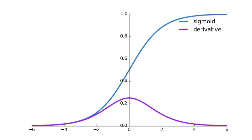
Output, Source: Author
Conclusion
Key Takeaways:
1 We covered the basic Introduction about Activation Function.
2 We also covered various needs to deploy the Activation Function.
3 We also covered the Python Implementation of Activation Functions
4 We also Covered various variants of the Activation Functions
5 At Last, we covered the need for the addition of Non-Linearity with Activation Functions
Read more blogs on Analytics Vidhya.
With this, I finish this blog.
My name is Pranshu Sharma and I am a Data Science Enthusiast
Thank you so much for taking your precious time to read this blog. Feel free to point out any mistake(I’m a learner after all) and provide respective feedback or leave a comment. Email: [email protected]
The media shown in this article is not owned by Analytics Vidhya and are used at the Author’s discretion.


