One Class Classification Using Support Vector Machines
This article was published as a part of the Data Science Blogathon.
Introduction
Classification problems are often solved using supervised learning algorithms such as Random Forest Classifier, Support Vector Machine, Logistic Regressor (for binary class classification) etc. A specific type of binary classification problem with single class training examples is called One-Class Classification (OCC). One-Class Classification is solved using an unsupervised or semi-supervised learning algorithm such as One-Class Support Vector Machines (1-SVM), Support Vector Data Description (SVDD) etc. One of the popular examples of One-Class Classification is Anamoly Detection (AD) i.e., outlier detection and novelty detection.
One Class Classification
One Class Classification (OCC) aims to differentiate samples of one particular class by learning from single class samples during training. It is one of the most commonly used approaches to solve Anamoly Detection (AD), a subfield of machine learning that deals with identifying anomalous cases which the model has never seen before. OCC is also called unary classification, class-modelling.
Overview of Support Vector Machines
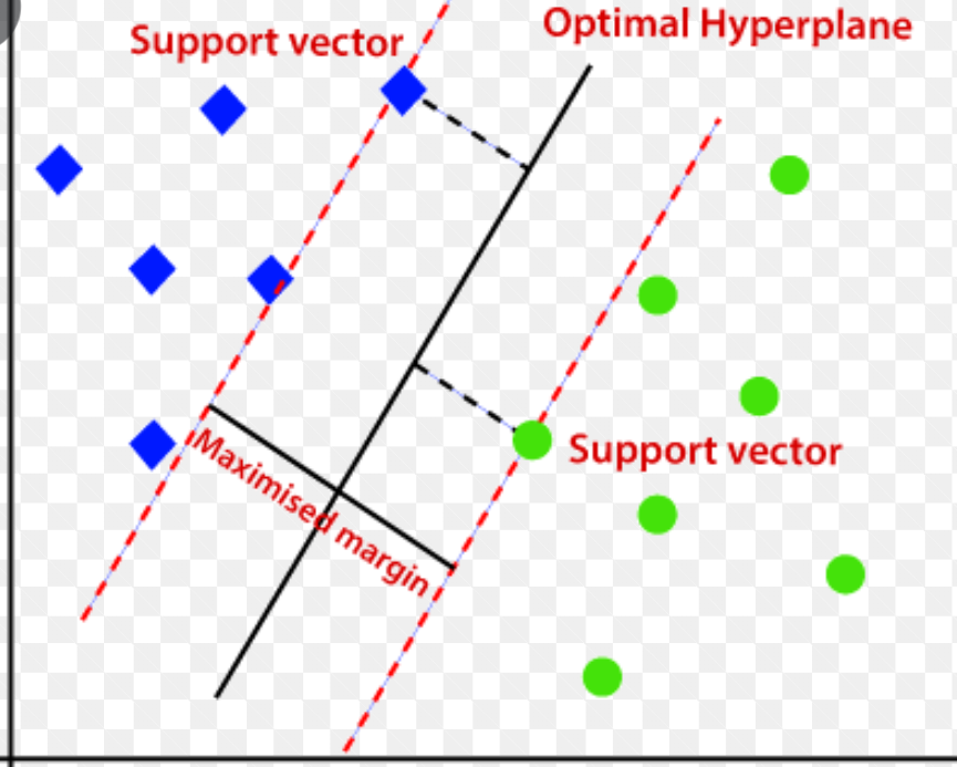
Support Vector Machines (SVMs) are one of the most robust statistical algorithms for classification and regression problem statements. SVMs (aka Support Vector Networks) are commonly used in classification problem statements due to their broader generalizability of unseen data. To understand SVMs more intuitively, let’s consider a dataset of positive (green balls), and negative examples (blue squares). As shown in the below figure, the aim is to draw the best fit line that would separate positive examples from negative examples but unlike linear classifiers, the best fit line drawn by SVM guarantees that the distance between the extreme points of both the classes towards the best fit line (or median) is almost equal and maximum. This idea of forming a gutter or widest street through learning makes SVMs robust during testing on unseen data. The SVM is already implemented on SK-learn directly from libsvm. The SVC can be imported to apply to any classification problem. More on this can be read here.
The function that is maximized to ensure the widest street is 2/|w| where w is a vector of random weights so that the function maximizes the street between support vectors. Maximizing 2/|w| is similar to minimizing the function 1/2*(|w|^2). In order to find the extremum of a function (1/2*(|w|^2)) with constraints i.e., there is a penalty if the function misclassifies any samples, Lagranges multiplier is applied. Applying Lagranges multiplier gives raise to a complex equation, which upon derivating w.r.t w gives the following relation
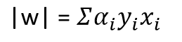
where w is a vector of weights, alpha is the Lagrange multiplier, y denotes either +1 or -1 i.e., class of the sample and x denotes the samples from data.
To better understand the mathematical derivation of the function for maximizing the gutter or street between the extreme samples of both positive and negative samples from the median or best fit line refer to the resources [1] and [2].
Source of the image: biss.co.in
One-Class Support Vector Machines
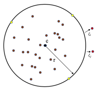
One-Class SVM is an unsupervised learning technique to learn the ability to differentiate the test samples of a particular class from other classes. 1-SVM is one of the most convenient methods to approach OCC problem statements including AD. 1-SVM works on the basic idea of minimizing the hypersphere of the single class of examples in training data and considers all the other samples outside the hypersphere to be outliers or out of training data distribution. The figure below shows the image that demonstrates the hypersphere formed by 1-SVM to learn the ability to classify out of training distribution data based on the hypersphere.
The mathematical expression to compute a hypersphere with centre c and radius r is
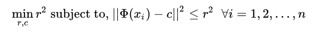
The expression above tries to minimize the radius of a hypersphere. However, the above formulation is very restrictive to outliers so, the more flexible formulation to tolerate outliers to an extent is given by
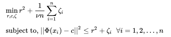
Here function phi is the hypersphere transformation of x samples. The figure below shows how the formulation of a hypersphere forms a hypersphere by minimizing the radius r, centre c.
1-SVM can be used for both kinds of anomaly detection applications i.e., outlier detection and novelty detection.
Images source: Wikipedia page on One-Class Classification (OCC).
Implementing 1-Support Vector Machines
Implementing 1-SVM is made very easy through SK-learn. The SK-learn implements the 1-SVM from libsvm. The SK-learn provides a class known as ‘OneClassSVM’ that internally implements the mathematical modelling of minimizing the hypersphere through training from data samples. To understand more about the mathematical reasoning behind the function that minimizes the hypersphere refer to the page.
In the below example, we train a One-Class SVM using random positive integers from 1 to 10. Further, the model is tested on a set of random positive and negative integers, the model successfully classifies the integers between positive and negative classes or samples.
Note: The One-Class SVM model treats the positive integers to be class +1 and negative integers to be -1. The samples in the training dataset are always considered positive samples by One-Class SVM.
>>> from sklearn.svm import OneClassSVM

>>> X = [[1],[2],[3],[4],[5],[6],[7],[8],[9],[10]]

>>> y = [[-1],[1],[-2],[2],[-3]]

>>> one_svm = OneClassSVM(gamma='auto', nu=0.01).fit(X)

>>> # gamma is used to set the kernel function for forming the hypersphere to learn and

>>> # differnciate samples and the hyperparameter nu is tuned to approximate the ratio

>>> # of outliers

>>> one_svm.predict(y)

[-1  1 -1  1 -1]


>>> # estimator predict method is used to classify the data points between classes 1, -1

>>> # based on the training data

>>> one_svm.score_samples(y)

array([1.24920628e-02, 8.32434204e-01, 8.38893433e-05, 8.32667829e-01, 7.64624773e-08])


>>> # score_samples method is used to access the scoring function of the estimator and the

>>> # contamination parameter is used to set the threshold for classification

>>> one_svm.decision_function(y)

array([-8.19890222e-01,  5.19198778e-05, -8.32298395e-01,  2.85544227e-04, -8.32382208e-01])


>>> # decision_function returns the value such that the negative values represents the

>>> # sample to be outlier or out of training distribution
Applications of One-Class Classification
One-Class Classification is very popularly used in Anamoly Detection (AD). AD is one of the challenging areas for Machine Learning Algorithms to generalize on. Some of the examples of AD are:
1. Outlier Detection: Detecting outliers from training data is an essential step of cleaning data before training a Machine Learning Model to ensure the robust performance of the model post-deployment in the real world.
2. AD in Acoustic Signals: One of the major applications of AD is to detect anomalies in industrial machinery using the Acoustic Signals generated by parts of machinery.
3. Novelty Detection and many others.
Conclusion
Understanding the 1-SVM helps to understand the problem statements that involve anomaly detection such as outlier detection, and novelty detection. There are some other semi-supervised and unsupervised learning algorithms for novelty detection, and outliers detection respectively. Some of the popular algorithms that can be implemented using SK-learn are Isolation Forest, Local Outlier Factor, and Robust Covariance.
Refer to the implementation of other techniques, from sklearn documentation to working on one-class classification problems to understand the difference between these techniques.
To compare the performance of these models, refer to the image here.
Understanding the mathematical reasoning behind the Support Vector Machines helps to better understand the ideas of One-Class SVMs. Refer to the articles/guide by Analytics Vidya on SVMs here. Stay tuned for the upcoming article on “Anamoly Detection in Acoustic Signals using VAEs and SVDD/1-SVM”. In the meantime explore the ideas of Support Vector Machines, 1-SVM, and SVDD from the articles of Analytics Vidya. Also, explore the VAEs, and their architecture from the article “An introduction to Autoencoders for Beginners” on Analytics Vidya here.
The media shown in this article is not owned by Analytics Vidhya and is used at the Author’s discretion.


