This article was published as a part of the Data Science Blogathon.
Why does a Machine Learning Model need to be interpretable?
In this article, I will walk you through one technique that makes any machine learning model interpretable. Generally, there is a misconception that only linear machine learning models are more interpretable than others. The Model explainability helps in decision making and gives clients reliability.

What is Explainability?
Explainability in AI is how much your features contribute or how important is your feature for the given output.
For Example,
If we have a linear model, feature importance is calculated by the magnitude of weights. If we have tree-based models, feature importance is calculated by Information gain or entropy. For deep learning models, we calculate using Integrated gradients.
Many of these AI systems are black-box, meaning we don’t understand how they work and why they make such decisions.
Can we have a model agnostic explainability?
A Research Paper named “Why Should I Trust You?” published by Marco Tulio Ribeiro, Sameer Singh, and Carlos Guestrin from the University of Washington in 2016 Link explains two techniques.
The two techniques are:
- LIME (Local Interpretable Model-agnostic Explanations)
- SHAP (SHapley Additive exPlanations)
In this blog, we will cover the in-depth intuition of the LIME technique.
Local Interpretable Model-agnostic Explanations (LIME)
LIME aims to identify an interpretable model over the interpretable representation that is locally faithful to the classifier.
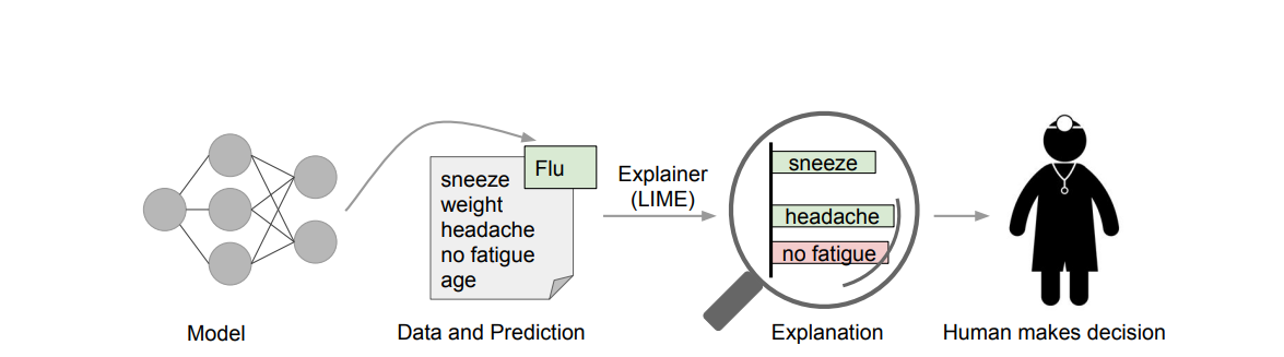
Source: https://arxiv.org/pdf/1602.04938.pdf
Local Interpretability answers the question, “Why is the model behaving in a specific way in the locality of a data point x ?”. LIME only looks at the local structure and not the global structure of the data.
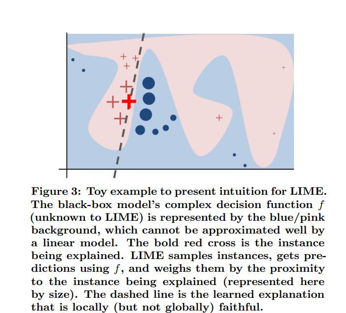
Source: https://arxiv.org/pdf/1602.04938.pdf
The high-level intuition is to consider the dark red + named X from the above diagram and take the data points neighboring X. From the above image, we can see that points closer to X have higher weightage and the points which are farther have lower weightage. Sample a bunch of points near X and fit a surrogate model g() (consider g () as Linear Model). The surrogate model approximates the f() model in the neighborhood of X. f() is the final black-box model, were given an input x, we’ll get the output y.
Let’s get into the mathematical intuition; for every X, there is another X’, where X’ is d’ dimension interpretable binary vector. For text data, the interpretable vector X’ is the presence or absence of a word (i.e.) Bag of Words. For Image data, the interpretable vector X’ is the presence or absence of an image patch or superpixel. Superpixel is nothing but a contiguous patch of similar pixels. For tabular data, if the feature is categorical, then X’ is the one-hot encoding of that feature, or if the feature is real-valued, then we do feature binning. The surrogate model g ∈ G is any interpretable model like linear models or Decision trees. The Ω(g) measures the complexity of the surrogate model. For example, the complexity increases as the number of non-zero weights increases in the linear model. Similarly, if the depth of the decision tree increases, the model complexity increases. The g is the function of X’.
Proximity Function
Πx(Z) = proximity measure between X and Z
where Πx is the locality of X
Local Fidelity and Interpretability
Local Fidelity means in the neighborhood of X, the surrogate function g() should closely resemble f().
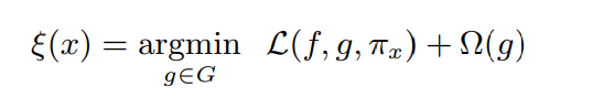
SOURCE: https://arxiv.org/pdf/1602.04938.pdf
The Loss function L(f, g, πx) shows how closely the function g() approximates f().
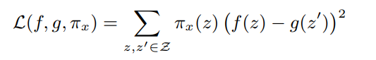
SOURCE: https://arxiv.org/pdf/1602.04938.pdf
Let Πx(z) = exp(−D(x, z)2 /σ2 ) be an exponential kernel.
g(z’) = wg ·z’
z’ is an interpretable feature corresponding to z.
Ω(g) represents K-Lasso, which means selecting the first K-features using Lasso Regularization.
Algorithm of LIME
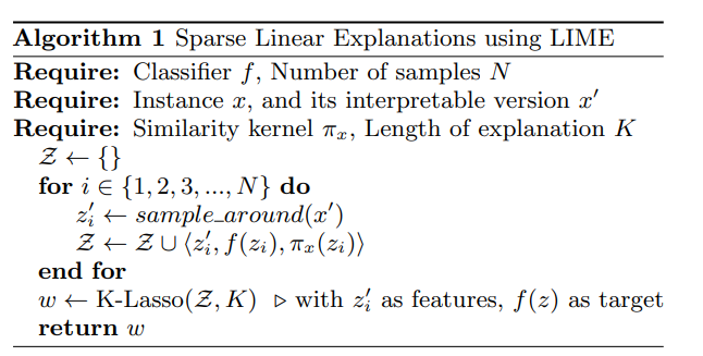
SOURCE: https://arxiv.org/pdf/1602.04938.pdf
Advantages of LIME
- Works well on Images, Text, and Tabular data.
- Model Agnostic
- K Lasso gives highly interpretable K features
Disadvantages of LIME
- Determining the right neighborhood Πx(z).
- Determining the correct kernel Width σ.
- The distance metric D(x, z) does not work well for high-dimensional data.
Code for Installing LIME
Install LIME using
pip install lime
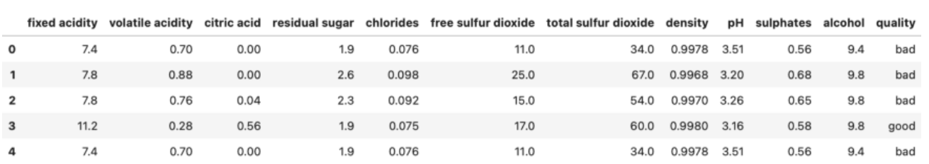
The data is split into train and test
from sklearn.model_selection import train_test_split
X = wine.drop('quality', axis=1)
y = wine['quality']
X_train, X_test, y_train, y_test = train_test_split(
    X, y, test_size=0.2, random_state=42)
For this example, we are using Random Forest Classifier.
from sklearn.ensemble import RandomForestClassifier
model = RandomForestClassifier(random_state=42)
model.fit(X_train, y_train)
score = model.score(X_test, y_test)
The Lime Library has a module named lime_tabular, which creates a tabular Explainer object. The parameters are:
- training_data – Training data must be in a Numpy array format.
- feature_names – Column names from the training set
- class_names – Distinct classes from the target variable
- mode – Classification in our Case
import lime
from lime import lime_tabular
explainer = lime_tabular.LimeTabularExplainer(
    training_data=np.array(X_train),
    feature_names=X_train.columns,
    class_names=['bad', 'good'],
    mode='classification')
The LIME library has an explain_instance function of the explainer object. The parameters required are:
- data_row – a single data point from the dataset
- predict_fn – a function used to make predictions
exp = explainer.explain_instance(
    data_row=X_test.iloc[1],
    predict_fn=model.predict_proba)
exp.show_in_notebook(show_table=True)
The show_in_notebook is used for data visualization
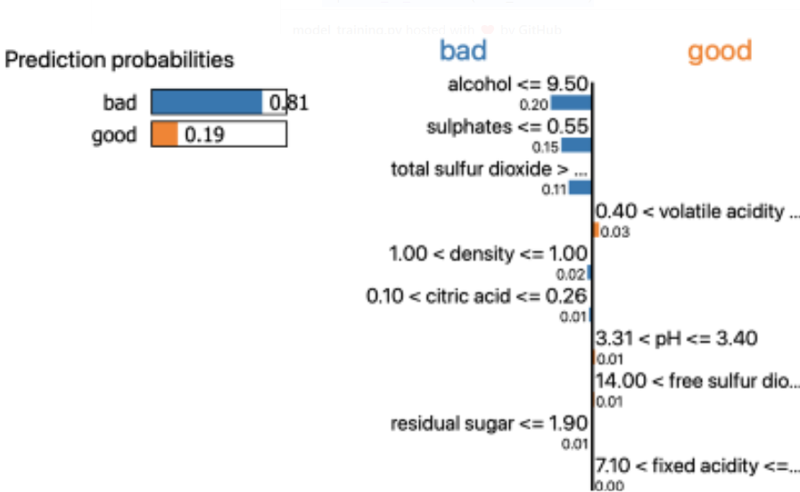
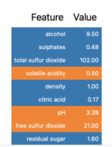
The above diagrams show that the random forest classifier is 81% confident that the data point belongs to the “bad” class. The values of alcohol, sulfates, and total sulfur dioxide elevate the chances of the data point being “bad.” There are different visualization techniques available in the LIME library.
Conclusion
- Congratulations! You’ve learned one of the techniques of the XAI Framework. The applications of Explainable AI(XAI) frameworks will continue to grow, enabling us to develop more robust and complex solutions in a ‘White-Box’ approach.
- XAI will enable both data scientists and stakeholders to understand complex data predictions. The LIME library also provides great visualization. By building such an interpretable model,s you gain acceptance and trust from the stakeholders.
- Besides LIME, examples of other explainable AI tools like IBM AIX 360, What-if Tool, and Shap can help increase the interpretability of the data and machine learning models.
The media shown in this article is not owned by Analytics Vidhya and is used at the Author’s discretion.


