This article was published as a part of the Data Science Blogathon.
Time series forecasting is the process of fitting a model to time-stamped, historical data to predict future values. It is an important machine learning analysis method with various use-cases, such as predicting the electricity consumption from the smart meters that can help the Electricity company plan the network expansion. Another example is to predict a city’s rainfall or solar irradiance based on historical data. This analysis can help the met department to take precautions and warn the citizens accordingly.
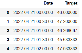
As the name suggests, time-series forecasting involves time series data gathered over a period, along with a variable we would like to forecast. For example, in our previous example of rainfall, we would need to have historical rainfall data for this week (any granularity like on a daily, hourly, min, sec basis) and the timestamp recorded against the rainfall. A sample of the data would look like this:
Source: https://quotesgram.com/img/forecast-quotes/5206570/
In the above example, the date is in the format of YYYY-MM-DD, and the time is in the 24-hour format. The target could be any variable you are assessing and want to predict. In our case, for example, it could be the rainfall in mm.
So, without spending more time on the details of Timeseries forecasting, let us start forecasting the demand of a product for the next ten months in the year, based on the historical data of five years, sampled daily.
The first step would be to initialize the essential libraries and import the data into the Jupyter Notebook.
 import numpy as np
 import pandas as pd
 from scipy import stats
 import statsmodels.api as sm
 import matplotlib.pyplot as plt
 import seaborn as sns
 from fbprophet import Prophet
After importing the necessary libraries, let’s see what our dataset looks like:
df=pd.read_csv("product15.csv")
df
We can see that there are 1131 rows corresponding to 1131 days of data. Ideally, the data should be 1825 rows, corresponding to 5 years of daily data (365*5=1825), but there are some days in the dataset where the demand for the product is unavailable. There could be multiple reasons for missing data, such as holidays, strikes, issues with data capturing, etc. This could impact our accuracy, but we will find a way to deal with the missing data later in this tutorial.
The next step is to assign the target and input variables to ‘y’ and ‘x’ respectively and visualize the dataset
x=data['Date']
y=data['demand']
plt.plot(x,y)
plt.title("Product 15 Demand over time")
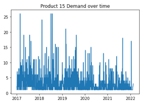
We can see that product 15’s demand is not following a pattern over the years. The demand was higher during 2017-2018, but from 2019, demand shows a downward trend, probably indicating the impact COVID-19 had on the demand.
Let’s ease our processing and resample the data on the monthly level to understand how the algorithm works. Also, we can always choose the resample the data on the hourly, daily, weekly, quarterly, and yearly levels to see different impacts resampling can have on the model’s performance.
monthly_data = data.resample('M',on='Date').mean()
monthly_data
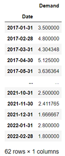
We can see that the number of rows has been reduced to 62, corresponding to 62 months of data. Demand has been averaged out for that particular month.

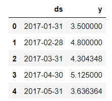
Before introducing the Facebook Prophet model to our code, we need to introduce a data frame df with two columns, ds and y. In this case, the ‘ds’ column would contain the time values, and ‘y’ would be our target variable, the product15 demand.
df = monthly_data.reset_index()
df.columns = ['ds', 'y']
df.head()
Now we will be initiating the Facebook Prophet Model(finally!). The function Prophet() needs to be called for this purpose and its optional seasonality. Later, we need to fit the model.
m = Prophet(weekly_seasonality=True,daily_seasonality=True)
m.fit(df)
Next, using the Facebook Prophet model, we want to predict Product 15’s demand for the next 10 months.
future = m.make_future_dataframe(periods=10,freq='m')
forecast = m.predict(future)
Here, inside the m.make_future_dataframe function, we can specify the number of periods we want the future dataset to be. Kindly note that these periods would be in addition to the existing dataset (m). For example, if we put periods=0, we would have our original dataset(m). We also need to specify the frequency at which we would like the future dataset to be. ‘m’ here denotes ‘monthly’ frequency. We can also have other frequencies such as ‘d’ for the day, ‘h’ for an hour, and so on. Let’s plot our forecasted values using the m.plot() command.
m.plot(forecast)
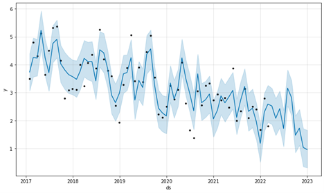
And BAZINGA! That’s it. The black dots represent our input data, product15’s historical demand values, and the solid blue lines represent the model’s predicted values. We can see that the model has done quite well predicting the values. That’s how easy it is to forecast a time series using Facebook Prophet Model. Compared to other time-series forecasting methods, such as LSTM, ARIMA/SARIMA, and Neural Networks, Facebook Prophet is quicker, simpler, and produces similar accuracy.
Next, we will be finding out the performance of our Facebook Prophet Model. We will use the conventional R-squared method to measure the model’s performance. Let us start by introducing the function first.
from sklearn.metrics import r2_score
original=df[['y']]
prediction=forecast[['yhat']]
r2_score(original,prediction)
print("Accuracy of the model is :",100*r2_score(original,prediction))

The model gave us a fair R2 score of 72%. We can improve the performance by various methods such as: adding holidays while initiating the Facebook Prophet function, resampling data into other frequencies such as hourly, daily, weekly, monthly, or quarterly, adding more seasonality to the data, and working on the ways to impute the missing values, etc.
We can conclude that time-series forecasting is one of the most important analyses with various use cases in different fields. There are various ways of forecasting time-series data, such as LSTM, AR, MA, ARIMA, and SARIMA, but we explored a relatively newer and simpler model called Facebook Prophet Model. This model does most of the processing, requires minimum user intervention, and produces accurate results that are at par with the other forecasting algorithms. The key takeaways of this article are:
The media shown in this article is not owned by Analytics Vidhya and is used at the Author’s discretion.
Lorem ipsum dolor sit amet, consectetur adipiscing elit,


