Informed Search Strategies for State Space Search Solving
This article was published as a part of the Data Science Blogathon.
Introduction
In the last article, we learned about various blind search algorithms because no further information is given beyond the constraints laid out in the problem. Hence, The algorithms look for traversing through many different states before reaching the goal state. The disadvantage of these search strategies is very poor Time complexity. Hence, The use of these strategies for solving real-world problems is non-sensical.
This solution can be overcome by providing some Heuristics i.e., ‘experience from exposure’ for solving this problem. This gives way to Informed Search Strategies. These algorithms promise a solution and can quickly solve any complex issue. They also have a lower time complexity.
Informed Search Strategies use some heuristic function to choose the node to ensure the most promising way to reach the goal. The most popular way to give the search problem more information about the problem is using heuristic functions. It is the cost estimate to reach the goal state from a particular node, n. Any problem-specific function is acceptable (arbitrary and nonnegative). H(n) = 0 if n is a goal node.
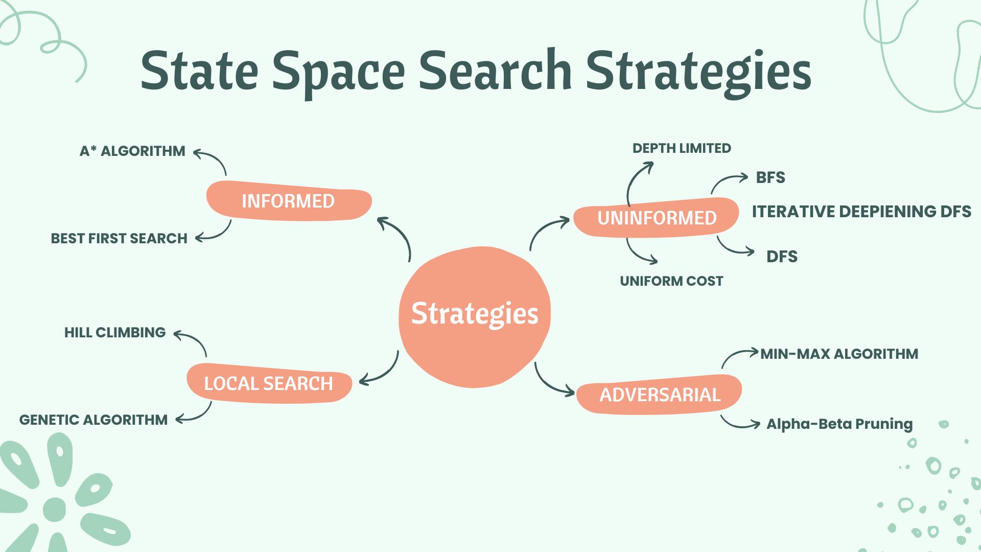
The two Informed Search strategies which we will see in this article are:
- Best First Search Algorithm
- A* Search Algorithm
Best First Search Algorithm
The Informed BFS follows a greedy approach for state transitions to reach a goal. For every node here, we maintain an evaluation function(f(n)) which provides a cost estimate. The idea is to expand the node with the lowest f(n) every time. The Evaluation function here has a heuristic function h(n) component. i.e.
f(n) = h(n)
The node that seems to be closest to the goal is therefore extended. The implementation of this algorithm is done using a priority queue ordered by the evaluation function for each node. The Pseudo code for the same would look like this:
function Best_First_Search(problem)
{
    node = problem.initial_state;
    frontier = priority queue with node as the only element
    explored = empty set
    loop(until goal state is found)
        if(frontier == empty)
            return failure
        node = frontier.pop()
        add node to explored_set
        if(node == problem.goal_state)
            return path from Initial state up to the node
        else
            generate successors of the node
        if(successors not in frontier and not in explored_set)
            add successor to the priority queue
    end loop
}
Properties of Best-First Search Algorithm:
Completeness: No. Gets stuck in a loop sometimes.
Space Complexity: O(b^m)
Time Complexity: O(b^m) (but a good heuristic can make a drastic improvement.)
Optimal: No
(b is the branching factor, and m is the maximum depth of the search space.)
A* Search Algorithm
A* Search Strategy is one of the most widely used strategies as it guarantees an optimal solution. The idea is to avoid expanding paths that are already expensive. On a similar grounds with Best-FS, It uses an evaluation function(f(n)) to evaluate every node(state) in the path.
f(n) = g(n) + h(n)
Where g(n) is the actual cost from the initial state to the current node.
h(n) is the estimated cost from the current node to the goal state.
A* algorithm succeeds in finding the shortest distance path for the problem in a faster time. Hence, It is the most widely accepted solution for state space search. The optimality of the solution for the A* search depends on the admissibility of the heuristic function we choose. We will learn more about it below in some time.
Algorithm for A* Search Strategy
Step1: Initialise an empty set(explored). Initialize a priority queue(frontier) ordered by the evaluation function of the nodes. Add the node(initial state) to the queue with its evaluation function, f(start) = 0+h(start) ………..(g(start)=0)
Step2: Loop until a goal is found – If the frontier is empty, return failure. Else, pop the node with the lowest evaluation function(best_node) from the frontier. Add the best_node to the explored set. Check if the best_node is the goal state; if yes, return the solution. Else, generate its successors.
Step3: For every successor generated, do
3.1: Set successor to point back to the best_node. (These backward links help find the solution path from the first state to the last goal state.)
3.2: Compute actual cost for successor, i.e. g(successor) = g(best_node) + actual cost from getting from best_node to the successor.
3.3: if the successor is already in frontier(i.e., a path already exists to reach this node), we call it old_node.
3.4: Add old_node to the list of best_node’s successors. Now, we will compare the actual cost(g(n)) for reaching the old_node via its previous path and the current new path(i.e., via best_node)
3.5: if the old path is cheaper, we continue. Else, we update the link of old_node’s parent to point to best_node and update the evaluation function of old_node.
3.6: if the successor is present in explored(i.e., we have visited this node before), we call it old_node. We repeat steps 3.4 and 3.5 to see if we get a new, better path. We must propagate the improvement to old_node’s successors.
3.7: if the successor is not in the frontier and not in the explored set, we add it to the frontier. Put it on the list of best_node’s successors. We compute its evaluation function,
(f(successor) = g(successor) + h(successor))
The time complexity for this algorithm is b^d.
The space complexity for this algorithm is b^d.
(where b is the branching factor of the tree and d is the depth of the solution node.)
The optimality of the solution depends on the admissible heuristics. So, what are admissible heuristics?
Admissible Heuristics
A heuristic function, h(n) is admissible if, for every node, h(n) is less than or equal to g(n). (here, g(n) is the actual cost to reach the goal state). Therefore, An admissible heuristic never overestimates the cost of reaching the goal. It is always optimistic about finding the best path to the goal node. If h(n) is admissible for the A* algorithm, we get the optimal solution to our problem.
If we have two admissible functions (h1 and h2), where h2(n) ≥ h1(n), we let h2 dominate over h1.
Conclusion
We learned about the two methods of informed search strategies in this essay. A heuristic function provides more information about the issue to the informed search strategies. We observed the algorithms for both tactics, i.e., Best-First Search and A* Search. According to their attributes, the A* algorithm is the most effective search strategy out of all the Informed and Uninformed Search strategies.
In the upcoming articles, we will learn about Local Search Algorithms and Constraint Satisfaction Problems for State Space Search. If you like my article, Connect with me on Linkedin here.
The media shown in this article is not owned by Analytics Vidhya and is used at the Author’s discretion.


