This article was published as a part of the Data Science Blogathon.
Introduction
Neural networks (Artificial Neural Networks) are methods or algorithms that mimic a human brain’s operations to solve a complex problem that a normal algorithm can’t solve.
A Perceptron in neural networks is a unit or algorithm which takes input values, weights, and biases and does complex calculations to detect the features inside the input data and solve the given problem. It is used to solve supervised machine-learning problems like classification and regression. It was designed as an algorithm, but its simplicity and accurate results are recognized as a building block of neural networks. We can also call it a machine learning model or a mathematical function.

Weights and biases (denoted as w and b) are the learnable parameters of neural networks. Weights are the parameters in a neural network that passes the input data to the next layer containing the weight of the information, and more weights mean more importance. Where bias we can consider as a linear line function effectively transposed by a constant value of bias.
Neurons are the basic unit of the artificial neural networks that receive and pass weights and biases from the previous layer to the next. In some complex neural network problems, we consider the increasing number of neurons per hidden layer to achieve higher accuracy values as the more the number of nodes per layer, the more information gained from the dataset. Still, after some values of nodes per layer, the model’s accuracy could not be increased. Then we should try other methods for getting higher accuracy values like increasing hidden layers, increasing the number of epochs, trying different activation functions and optimizers, etc.
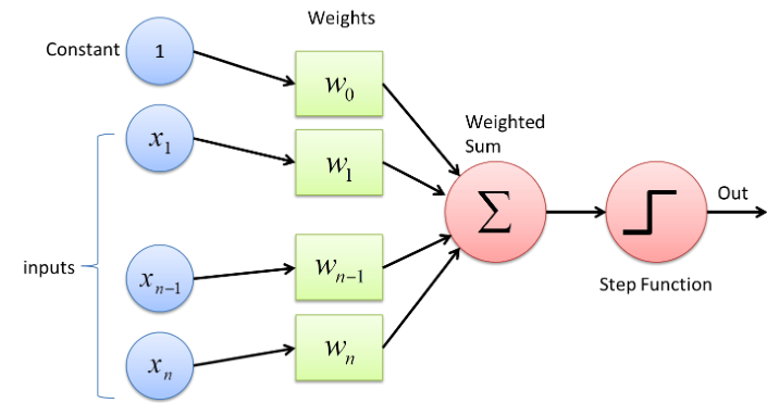
Above is the simple architecture of a perceptron having Xn inputs and a constant. Each input will have its weight, and the constant will be its weight (W0) or bias (b). These weights and biases will be passed into Summation ( Sigma ), and then it will pass to an activation function (In this case, Step Function), which will give us a final output for the data fed.
Here the summation of weights and biases is going into an activation function as input. The summation function will look like this:
Z = W1X1 + W2X2 + b
Now the activation function will take Z as input and bring it into a particular range. Different Activation functions use different functions for this process.
Multi-Layer Perceptrons
The only problem with single-layer perceptrons is that it can not capture the dataset’s non-linearity and hence does not give good results on non-linear data. This problem can be easily solved by multi-layer perception, which performs very well on non-linear datasets.

Fully connected neural networks (FCNNs) are a type of artificial neural network where the architecture is such that all the nodes, or neurons, in one layer are connected to the all neurons in the next layer.
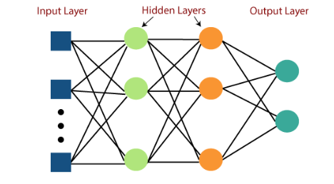
A Multi-layer Perceptron is a set of input and output layers and can have one or more hidden layers with several neurons stacked together per hidden layer. And a multi-layer neural network can have an activation function that imposes a threshold, like ReLU or sigmoid. Neurons in a Multilayer Perceptron can use any arbitrary activation function.
In the above Image, we can see the fully connected multi-layer perceptron having an input layer, two hidden layers, and the final output layer. The increased number of hidden layers and nodes in the layers help capture the non-linear behavior of the dataset and give reliable results.
MLP Notations
The most difficult thing to understand while working with neural networks is the back-propagation algorithm we used to train a neural network to update weights and biases recursively and reach the highest accuracy.
Now while training a neural network, there are lots of weights and biases exits in a neural network, and a back-propagation is also a process of updating weights and biases, so notations of all different weights and biases become a pre-requisite to understanding core intuition of the back-propagation of the neural networks.

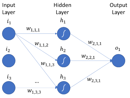
The above picture shows the Multi-layer neural network having an input layer, a hidden layer, and an output layer.
1. Notation for Weights :
Notation: Wijh
where,
i = From which node weight is passing to the next layer’s node.
j= To which node weight is arriving.
h = Layer in which weight is arriving.
Example:
W111 = Weight passing into 1st node of 1st layer of 1st node of the previous layer.
W231 = Weight passing into the 3rd node of the 1st hidden layer from the 2nd node of the previous layer.
W451 = Weight passing into the 5th node of the 2nd hidden layer from the 4th node of the previous layer.
2. Notations for Biases :
Notation: bij
Where,
i = Layer to which a bias belongs.
j = node to which a bias belongs.
Example:
b11 = biases of 1st node of 1st hidden layer.
b23 = bias of 3rd of 2nd hidden layer.
b41 = bias of 1st node of 4th hidden layer.
3. Notations for Outputs:
Notation: Oij
Where,
i = Layer to which a bias belongs.
j = node to which a bias belongs.
Example:
O11 = Output of 1st node of 1st hidden layer.
O45 = Output of 5th of 4th hidden layer.
O34 = Output of 4th node of 3rd hidden layer.
Calculating Total Trainable Parameters
Total Trainable Parameters for a given between 2 layers of an artificial neural network is a sum of total weights and total biases that exist between them.

Total Trainable Parameters Between two layers in a Neural Network = [ Number of Nodes in the first layer * Number of nodes in the second layer ] (Weights) + [ Number of nodes in the second layer ] (Biases)
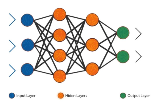
1. Trainable Parameters Between the Input layer and First Hidden Layer:
weights = 3 * 4 = 12
biases = 4 (4 nodes in 1st hidden layer)
Trainable Parameters = weights + biases
= 12 + 4
= 16
2. Trainable Parameters Between First Hidden layer and Second Hidden Layer:
weights = 4 * 2 = 8
biases = 2 (2 nodes in 1st hidden layer)
Trainable Parameters = weights + biases
= 8 + 2
= 10
3. Trainable Parameters Between Second Hidden layer and Output Layer:
weights = 2 * 2 = 4
biases = 2 (2 nodes in 1st hidden layer)
Trainable Parameters = weights + biases
= 4 + 2
= 6
Conclusion
In this article, we first studied some basic concepts of neural networks, perceptrons, multi-layer perceptrons, and methods for calculating the total trainable parameters of the neural networks, including notations of weights, biases, and outputs in multi-layer perceptrons. Knowledge about this key concept will not only help avoid some misconceptions of a person regarding neural networks but also help understand some core concepts of neural networks (e.g., backpropagation).
Key Insights are:
1. Perceptrons are the fundamental building block of neural networks having simple and easily understandable architecture.
2. Multi layers perceptrons can be used where perceptrons fail due to the nonlinearity of the dataset.
3. Notations of input, outputs, and weights should be known to each person working with neural networks to avoid misconceptions in understanding neural network architectures.
4. Total trainable parameters can be calculated for single or multiple hidden layers to get a clear idea of the parameters included in a particular neural network.
The media shown in this article is not owned by Analytics Vidhya and is used at the Author’s discretion.


