Optimization Essentials for Machine Learning
Overview
There are 4 mathematical pre-requisite (or let’s call them “essentials”) for Data Science/Machine Learning/Deep Learning, namely:
- Probability & Statistics
- Linear Algebra
- Multivariate Calculus
- Convex Optimization
Table of contents
- Overview
- Why should I bother about Optimization in ML?
- Where is Optimization used in DS/ML/DL?
- What are Convex Functions?
- What is optimization, and how is it different from other mathematical problems?
- What are the Different types of Optimization Problems?
- How do we “Solve” the Optimization Problems?
- Which Approach should be used to Solve What kind of Optimization Problem?
- Finally, let’s see “Optimization in Action”
- 9. Where else is Optimization used in Machine Learning & Deep Learning?
- 10. Other Applications of Optimization
- Conclusion
Why should I bother about Optimization in ML?
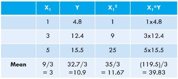
In fact, behind every Machine Learning (and Deep Learning) algorithm, some optimization is involved. Ok, let me take the simplest possible example. Consider the following 3 data points:
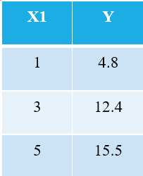
Everyone familiar with machine learning will immediately recognize that we are referring to X1 as the independent variable (also called “Features” or “Attributes”), and the Y is the dependent variable (also referred to as the “Target” or “Outcome”). Hence, the overall task of any machine is to find the relationship between X1 & Y. This relationship is actually “learned” by the machine from the DATA, and hence we call the term Machine Learning. We, humans, learn from our experiences, similarly, the same experience is fed into the machine in the form of data.
Now, let’s say that we want to find the best fit line through the above 3 data points. The following plot shows these 3 data points in blue circles. Also shown is the red line (with squares), which we are claiming as the “best-fit line” through these 3 data points. Also, I have shown a “poor-fitting” line (the yellow line) for comparison.
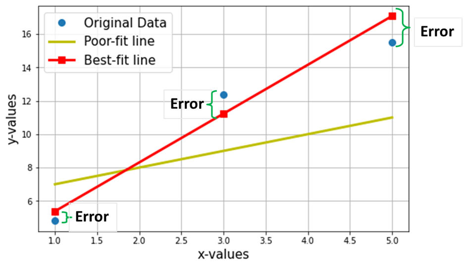
The net Objective is to find the Equation of the Best-Fitting Straight Line (through these 3 data points, mentioned in the above table).
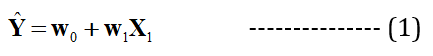
is the equation of the best-fit line (red-line in the above plot), where w1 = slope of the line; w0 = intercept of the line.
In machine learning, this best-fit is also called the Linear Regression (LR) model, and w0 and w1 are also called model weights or model coefficients.
The predicted values from the Linear Regression model (Y^) are represented by red-squares in the above plot. Of course, the predicted values are NOT exactly the same as the actual values of Y (blue circles), the vertical difference represents the error in the prediction given by:

for any ith data point.
Now I claim that this best fit-line will have the minimum error for prediction (among all possible infinite random “poor-fit” lines). This total Error across all the data points is expressed as the Mean Squared Error (MSE) Function, which will be minimum for the best-fit line.
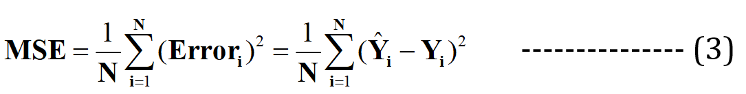
N = Total no. of data points in the dataset (in the current case, it is 3)
Minimizing or maximizing any quantity is mathematically referred to as an Optimization Problem, and hence the solution (the point where the minimum/maximum exists) is referred the optimal values of the variables.
Where is Optimization used in DS/ML/DL?
There are two types of Supervised learning tasks: Regression & Classification.
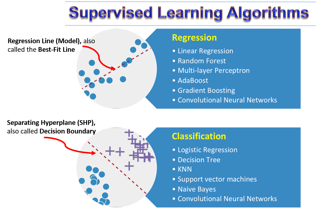
In Regression problems, the objective is to find the “best-fit” line passing through the majority of the data points (basically the best-fit line will capture the pattern/relationship between X & Y), and will have the minimum value of an error function (also called as the Cost function or Loss function), commonly which is the Mean Square Error (MSE). Why only MSE, why not a simple sum of errors terms or mean the absolute error will be discussed in another article. Hence, as discussed in the above section, the net objective is to find the line having the minimum value of this error function. The following table lists the Error functions being minimized in the most commonly used regressor algorithms.
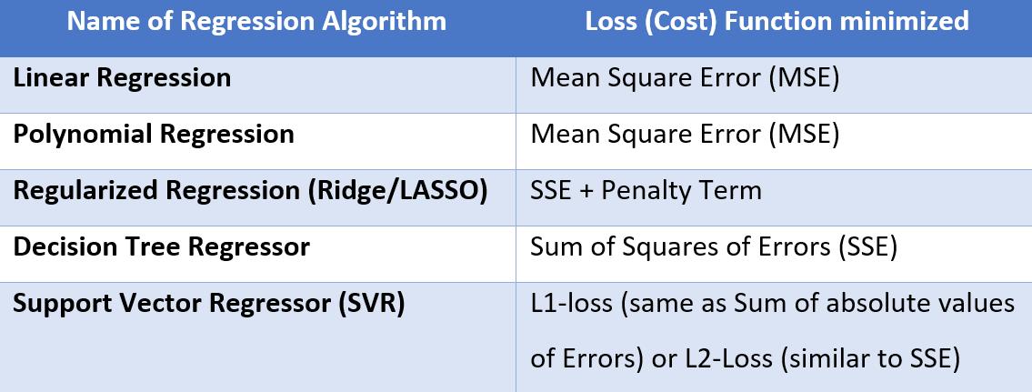
Apart from the above list, a few ML & DL algorithms also use Huber loss.
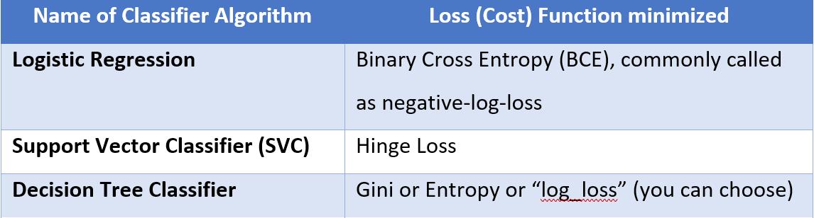
In Classification Problems, the objective is to find the “best-separating” Hyperplane, essentially a line (or a curve) passing “between” the data points, such that it is able to separate the majority of the data points into 2 or more classes. In such cases, we want to minimize the Classification error (for wrongly-labeled data points). This classification error is expressed again in many forms depending upon the type of Classifier (ML) algorithm, and the same has been summarized in the table below.
In Deep Learning architectures, in fact, you can create your customized neural networks and choose your Loss function as per the problem (all available loss functions are listed in this link: https://keras.io/api/losses/)
What are Convex Functions?
Now that we have a fair idea that optimization deals with maximizing or minimizing a quantity, the basic question can any mathematical function be maximized or minimized? The simple answer is NO. Mathematical functions are strictly monotonous and don’t have any maxima/minima. (e.g. the square function y = x^2 or the exponential function y=e^x).
Convex functions have minima (within a given range), whereas strict convex functions will have exactly one minimum (in the entire range). Examples of convex functions of a single variable include the quadratic function (x^2) and the exponential function (e^x). In machine learning, we prefer that the Loss functions are not only convex but also continuous and differentiable. For example, the loss function for LASSO regression (SSE + lambda*L1-Norm) is convex, whereas that of Ridge regression (MSE/SSE + lambda*square of L2-norm) is strictly convex, similar to the MSE loss function used in Linear Regression.
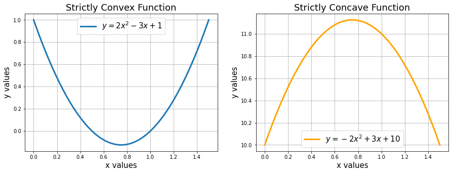
Similarly, the concave function will have maxima. You can read more about convex & concave functions here.
What is optimization, and how is it different from other mathematical problems?
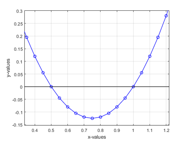
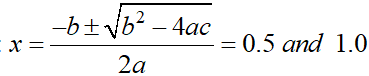
Consider the problem of finding the roots of the polynomial 2x^2 – 3x + 1. The roots of a polynomial represent the values of x, for which the f(x) = 0. You can see from the above plot that the roots are 0.5 & 1.0. Such kind of “deterministic” problems are not considered optimisation problems.
Any problem that deals with maximizing or minimizing any physical quantity (which can be mathematically computed/expressed in the form of some variables) are defined as an Optimization Problem.
Mathematically,
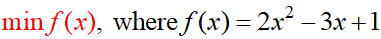
is read as “find the minimum value of f(x)”, is an optimization problem. Here f(x) is called the Objective function (which is referred to as the Loss function or Cost Function in our machine learning), and the variable “x” here is called the “Decision Variable”.
Also the below
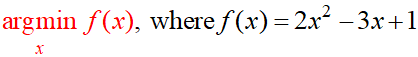
is read as “find the argument x for which f(x) has minimum value”, is also an optimization problem. ALL our machine-learning optimizations are of this type!
What are the Different types of Optimization Problems?
There are 2 types of Optimization Problems in general: Constrained & Unconstrained.
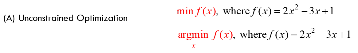
Where there are neither any “bounds” on the values of x (e.g. x has to be a positive number, or it should be between 0 & 10, etc.) nor any type of constraints that need to be satisfied.
Linear Regression is an example of unconstrained optimization, given by:
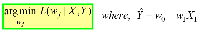
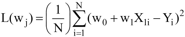
Says, Find the optimal weights (wj) for which the MSE Loss function (given in eq. 3 above) has min value, for a GIVEN X, Y data (refer to very first the table at the start of the article). L(wj) represents the MSE Loss, a function of the model weights, not X or Y. Remember, X & Y is your DATA and is supposed to be CONSTANT! The subscript “j” represents the jth model coefficient/weight.
(B) Constrained Optimization: for example
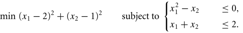
says “minimize (x1-2)^2 + (x2-1)^2, subject to the constraints” as given above.
The range of values of the decision variable which satisfy all the constraints constitutes the “Feasible Region”, and the final optimal value will lie in these feasible regions. If the constraints are very “hard” and contradicting, there may not be any “feasible solution” to the given optimization problem.
An example of constrained optimization is Support Vector Machines (SVM), which is an ML algorithm typically used for classification (although it has a regressor variant too). By default, the Support Vector Classifier (SVC) tries to find a separating hyperplane with maximum margin, with a “hard constraint” that all the data points must be classified correctly. However, if the data is not linearly separable, it may not lead to any solution. In such cases, we use the “Kernel Trick” and/or use the soft-margin variant of SVM (controlled by the hyperparameter C in the algorithm), with the loss function being Hinge Loss. Further details about the SVM problem formulation, loss function, and the Kernel Trick can be found in this article on SVM algorithm.
How do we “Solve” the Optimization Problems?
Typically there are 2 approaches to solving most of the most complex numerical/scientific problems:
- Analytical Method: This is the “pen-and-paper” theoretical method normally taught to us in usual school/university syllabi. These methods will give the “exact” solution for any well-posed mathematical problem which is solvable. For example, if we are asked to find the values of x for which the function f(x) = 2x^2 – 3x + 1 values equal to zero (normally called the “roots” of the polynomial), we know have been taught to solve for the roots of a generic 2-degree polynomial ax^2 + bx + c = 0, given by:
- Numerical Methods Approach: Normally, in this approach, we start with a guess value as the solution and then perform some calculations (in this case, evaluate the function f(x), and then “improve” the solution with every iteration until we get the desired result (called as Convergence). For example, if the tolerance is set to 0.0001, then the iterations will stop when the value of the f(x) <= 0.0001, and the whole optimization process is said to have Converged to an optimal solution. Typical “zero-finding” numerical methods include Newton’s, Secant, Brent’s, and Bisection. You can also solve differential equations iteratively using Euler’s and Finite Difference methods. I would suggest an awesome book titled Numerical Method for Engineers by Steven Chapra for studying this topic in detail.
Similarly, for solving the optimization problems, we again have 2 approaches:
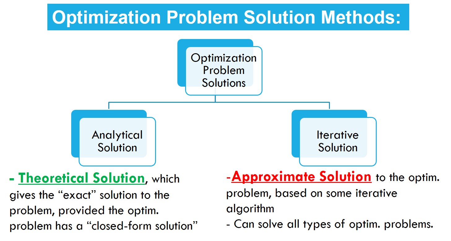
- Analytical method: One example of this is the Ordinary Least Squares Method (OLS), used by the LinearRegression class of the scikit-learn package in Python and the numpy polyfit function. As previously mentioned, the OLS technique gives the best-fit line’s exact coefficients (slopes and intercept terms).
- Iterative Solution: The most popular iterative method for solving the optimization problems in machine learning is the Gradient Descent Algorithm and its variants, Stochastic Gradient Descent and the MiniBatch Gradient Descent. There are also more advanced variants used in Deep Learning such RMSprop, Adam, Adadelta, Adagrad, Adamax & Nadam (refer to this webpage from Keras. There are several articles on Gradient Descent on our Analytics Vidhya Blog.
Apart from the GD-based methods, there are other iterative methods to solve constrained and unconstrained optimization problems (refer to the SciPy documentation page:
The iterative solvers also include a category of “Heuristic” solvers like Genetic Algorithms, Particle Swarm Optimization (PSO), Ant Colony Optimization (ACO), and other non-greedy algorithms like Simulated Annealing (SA).
Which Approach should be used to Solve What kind of Optimization Problem?
For Unconstrained minimization, you can use methods like the Conjugate Gradient (CG), Newton’s Conjugate Gradient, or the quasi-Newton method of Broyden, Fletcher, Goldfarb, and Shanno algorithm (BFGS), Dog-leg Trust-region algorithm, Newton Conjugate Gradient Trust-region algorithm, or the Newton GLTR trust-region algorithm.
Do I need to know all of this? Well, some of these techniques are used in ML algorithms! For example, the LogisticRegression class of the scikit-learn library uses the BFGS algorithm by default.
Similarly, for Constrained optimization problems with and without bounds, we have algorithms like Nelder-Mead, Limited-memory BFGS (called L-BFGS), Powell’s method, Truncated Newton’s Conjugate Gradient algorithms, Sequential Least Squares Programming (SLSQP) etc.
Finally, let’s see “Optimization in Action”
(A) OLS Method:
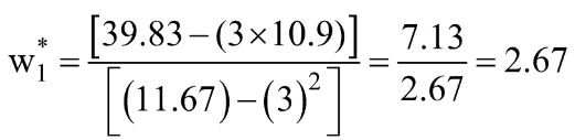
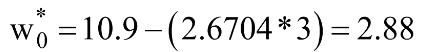
Coming back to our sample dataset, which I presented at the start of the article, upon substituting for Y^ in eq. 3, the final MSE Loss Function looks as:
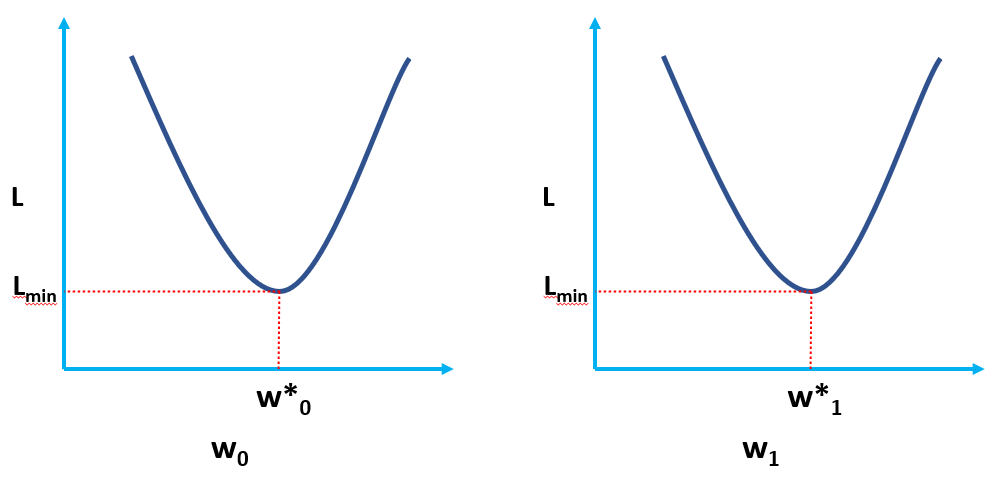
Clearly, L is a function of model weights (w0 & w1), whose optimal values we have to find upon minimizing L. The optimal values are represented by (*) in the figure below.
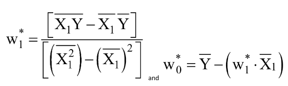
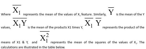
Without going into the derivations in this article (planned in a follow-up article), the final optimal values of w0 & w1 (where the MSE Loss function is minimum) are given by:
Let us calculate the same using Python code:
import numpy as np

# define your X and Y as NumPy Arrays
X = np.array([1,3,5])
Y = np.array([4.8,12.4,15.5])

# np.polyfit function does a 1-dimensional Polynomial fitting
# and the np.poly1d function convers the polynomial coefficents
# into a polynomila object that can be evaluated
p = np.poly1d(np.polyfit(X,Y,1))
print(p)
[OUTPUT]: 2.675 x + 2.875
You can see our “hand-calculated” values match very closely the values of slope and intercept obtained using NumPy (small difference is due to round-off errors in our hand-calculations). We can also verify that the same OLS is “running behind the scenes” of the LinearRegression class from the scikit-learn package as demonstrated in the code below.
# import the LinearRegression class from scikit-learn package
from sklearn.linear_model import LinearRegression

LR = LinearRegression() # create an instance of the LinearRegression class

# define your X and Y as NumPy Arrays (column vectors)
X = np.array([1,3,5]).reshape(-1,1)
Y = np.array([4.8,12.4,15.5]).reshape(-1,1)

LR.fit(X,Y) # calculate the model coefficients
LR.intercept_ # the bias/intercept term (w0*)
[Output]: array([2.875])LR.coef_ # the slope term (w1*)
[Output]: array([[2.675]])
(B) Iterative Methods for solving optimization problems
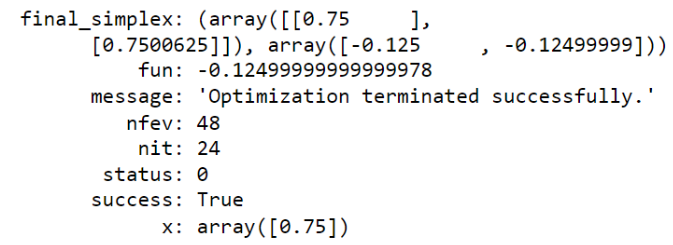
Let me demonstrate this using an example from Section 4, where I defined a function fx=2*x^2 – 3*x +1 and plotted it. If you see the plot, there seems to be a minima between 0.7 & 0.8.
fx = lambda x: 2*x**2 - 3*x + 1from scipy.optimize import minimize
x0 = 0 # rough guess about the minima (can be obtained from the plot initially)
soln = minimize(fx, x0)
soln
Output:
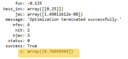
soln.x # see this is our "approximate solution" (minima) from the iterative solver,
# against the theoretical solution of 0.75.
[Output]: array([0.74999999])
You can also see the value of the function at minima is -0.125. Another example code below using the Nelder-Mead method:
soln = minimize(fx, x0, method='Nelder-Mead')
soln
Output:
9. Where else is Optimization used in Machine Learning & Deep Learning?
Okay, we have a fair idea about optimization by now. Now let us see where all this is used in ML & DL.
- Linear Regression uses the OLS method for solving the optimal model coefficients.
- In Logistic Regression, the optimal values of the model coefficients are obtained by minimizing the BinaryCrossEntropy Loss function. The Logistic Regression class of scikit-learn uses the “solver” option (default value of ‘lbfgs’) and “max_iter” (default value of 100) as one of the hyperparameters. Clearly, the LogisticRegression class in sklearn uses iterative solvers, and the other supported solvers are ‘liblinear’, ‘sag’, ‘saga’ and ‘newton-cg’. A detailed explanation of these solvers can be read from here:
- In Support Vector Machines, we are minimizing the Hinge loss. The Python implementation in scikit-learn API uses the solvers from the “LIBSVM” library (coded in C language).
- In Deep Learning, we normally use the advanced variants of the MiniBatch Gradient Descent algorithm such RMSprop, Adam, Adadelta, Adagrad, Adamax & Nadam (refer to this webpage from Keras ) to train our neural networks.
10. Other Applications of Optimization
Apart from the Data Science domain, optimisation problems are abundant in the industry. Think of a manufacturing company trying to minimize the cost of manufacturing a product to maximize its profit. This total cost will be a function of the manpower cost, raw materials cost, costs of inventory, storage, transportation and other logistics. And furthermost of these variables come along with their own set of constraints. So you can find the “optimal number of units” to be manufactured to have minimum manufacturing cost.
Another associated example is finding the optimal sequence of the operations in a manufacturing process or assembly unit, such that the machines are optimally used (machine idle time is minimized, and some are not over-utilized, while other parts are kept in waiting). This is a scheduling problem (with constraints).
Another example of a scheduling problem is finding the optimal timetable (occupancy and/or availability table) of employees in a company for doing specific tasks in different shifts so that the manpower cost is minimized, and overtime pay may not be needed.
Another widespread problem is Vehicle Routing with capacity constraints. This is more of a transportation problem in civil engineering, where we have to find the optimal route so that the traffic congestion is minimum. Also, the time a traffic signal remains open/closed has to be optimal. Another associated example is Vehicle Routing Problem with pickup and delivery constraints, which may include time window constraints. Think of a courier delivery boy who has been given a target collecting and dropping 20 parcels every day in a given geographic location. He/she wants to find the optimal route with minimal traffic, shortest distance, minimum time taken and doesn’t want to visit the same locality twice (another very similar example is the classical Travelling Salesman problem.
Chemical engineers, want to have the optimal design (shape, size, diameter, length etc.) of the pressure vessels for chemical reactions, boilers, and pipes for transporting the fluids and even storage.
Some typical applications from different engineering disciplines are mentioned below (reproduced from page 5 of the book Engineering Optimization: Theory and Practice by Singiresu S. Rao) :
1. Design of aircraft and aerospace structures for minimum weight
2. Finding the optimal trajectories of space vehicles
3. Design of civil engineering structures such as frames, foundations, bridges, towers, chimneys, and dams for minimum cost
4. Minimum-weight design of structures for earthquake, wind, and other types of random loading
5. Design of water resources systems for maximum benefit
6. Optimal plastic design of structures
7. Optimum design of linkages, cams, gears, machine tools, and other mechanical components
8. Selection of machining conditions in metal-cutting processes for minimum production cost
9. Design of material handling equipment, such as conveyors, trucks, and cranes, for minimum cost
10. Design of pumps, turbines, and heat transfer equipment for maximum efficiency
11. Optimum design of electrical machineries such as motors, generators, and transformers
12. Optimum design of electrical networks
13. Shortest route was taken by a salesperson visiting various cities during one tour
14. Optimal production planning, controlling, and scheduling
15. Analysis of statistical data and building empirical models from experimental results to obtain the most accurate representation of the physical phenomenon
16. Optimum design of chemical processing equipment and plants
17. Design of optimum pipeline networks for process industries
18. Selection of a site for an industry
19. Planning of maintenance and replacement of equipment to reduce operating costs
20. Inventory control
21. Allocation of resources or services among several activities to maximize the benefit
22. Controlling the waiting and idle times and queueing in production lines to reduce the costs
23. Planning the best strategy to obtain maximum profit in the presence of a competitor
24. Optimum design of control systems
Conclusion
There are several Python packages for solving optimization problems like CPLEX, DOCPLEX, PULP, PYOMO, ORTOOLS, PICOS, CVXPY, GUROBI, LOCALSOLVER etc. I hope this article has given enough motivation to dive deeper into the concept and applications of Optimization. More to be discussed in further articles.
If you liked my article or have any questions, please post a comment below.


Very nicely explained, I was looking for a comprehensive article to teach optimization and found this to be very useful. many thanks.