Introduction
In this article, I’ll show you the application of kNN (k – nearest neighbor) algorithm using R Programming. But, before we go ahead on that journey, you should read the following articles:
- Basics of machine learning from my previous article
- Common machine learning algorithms
- Introduction to kNN – simplified
We’ll also discuss a case study which describes the step by step process of implementing kNN in building models.
This algorithm is a supervised learning algorithm, where the destination is known, but the path to the destination is not. Understanding nearest neighbors forms the quintessence of machine learning. Just like Regression, this algorithm is also easy to learn and apply.

What is kNN Algorithm?
Let’s assume we have several groups of labeled samples. The items present in the groups are homogeneous in nature. Now, suppose we have an unlabeled example which needs to be classified into one of the several labeled groups. How do you do that? Unhesitatingly, using kNN Algorithm.
k nearest neighbors is a simple algorithm that stores all available cases and classifies new cases by a majority vote of its k neighbors. This algorithms segregates unlabeled data points into well defined groups.
How to select appropriate k value?
Choosing the number of nearest neighbors i.e. determining the value of k plays a significant role in determining the efficacy of the model. Thus, selection of k will determine how well the data can be utilized to generalize the results of the kNN algorithm. A large k value has benefits which include reducing the variance due to the noisy data; the side effect being developing a bias due to which the learner tends to ignore the smaller patterns which may have useful insights.
The following example will give you practical insight on selecting the appropriate k value.
Example of kNN Algorithm
Let’s consider 10 ’drinking items’ which are rated on two parameters on a scale of 1 to 10. The two parameters are “sweetness” and “fizziness”. This is more of a perception based rating and so may vary between individuals. I would be considering my ratings (which might differ) to take this illustration ahead. The ratings of few items look somewhat as:
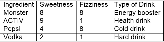
“Sweetness” determines the perception of the sugar content in the items. “Fizziness” ascertains the presence of bubbles in the drink due to the carbon dioxide content in the drink. Again, all these ratings used are based on personal perception and are strictly relative.
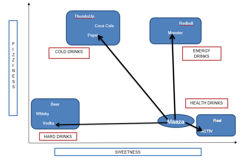
From the above figure, it is clear we have bucketed the 10 items into 4 groups namely, ’COLD DRINKS’, ‘ENERGY DRINKS’, ‘HEALTH DRINKS’ and ‘HARD DRINKS’. The question here is, to which group would ‘Maaza’ fall into? This will be determined by calculating distance.
Calculating Distance
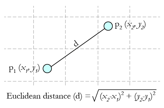
Now, calculating distance between ‘Maaza’ and its nearest neighbors (‘ACTIV’, ‘Vodka’, ‘Pepsi’ and ‘Monster’) requires the usage of a distance formula, the most popular being Euclidean distance formula i.e. the shortest distance between the 2 points which may be obtained using a ruler.
 Source: Gamesetmap
Using the co-ordinates of Maaza (8,2) and Vodka (2,1), the distance between ‘Maaza’ and ‘Vodka’ can be calculated as:
dist(Maaza,Vodka) = 6.08
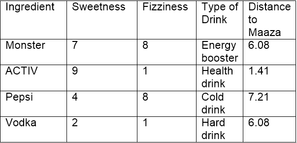
Using Euclidean distance, we can calculate the distance of Maaza from each of its nearest neighbors. Distance between Maaza and ACTIV being the least, it may be inferred that Maaza is same as ACTIV in nature which in turn belongs to the group of drinks (Health Drinks).
If k=1, the algorithm considers the nearest neighbor to Maaza i.e, ACTIV; if k=3, the algorithm considers ‘3’ nearest neighbors to Maaza to compare the distances (ACTIV, Vodka, Monster) – ACTIV stands the nearest to Maaza.
kNN Algorithm – Pros and Cons
Pros: The algorithm is highly unbiased in nature and makes no prior assumption of the underlying data. Being simple and effective in nature, it is easy to implement and has gained good popularity.
Cons: Indeed it is simple but kNN algorithm has drawn a lot of flake for being extremely simple! If we take a deeper look, this doesn’t create a model since there’s no abstraction process involved. Yes, the training process is really fast as the data is stored verbatim (hence lazy learner) but the prediction time is pretty high with useful insights missing at times. Therefore, building this algorithm requires time to be invested in data preparation (especially treating the missing data and categorical features) to obtain a robust model.
Case Study: Detecting Prostate Cancer
Machine learning finds extensive usage in pharmaceutical industry especially in detection of oncogenic (cancer cells) growth. R finds application in machine learning to build models to predict the abnormal growth of cells thereby helping in detection of cancer and benefiting the health system.
Let’s see the process of building this model using kNN algorithm in R Programming. Below you’ll observe I’ve explained every line of code written to accomplish this task.
Step 1- Data collection
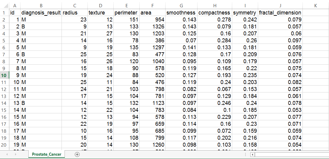
We will use a data set of 100 patients (created solely for the purpose of practice) to implement the knn algorithm and thereby interpreting results .The data set has been prepared keeping in mind the results which are generally obtained from DRE (Digital Rectal Exam). You can download the data set and practice these steps as I explain.
The data set consists of 100 observations and 10 variables (out of which 8 numeric variables and one categorical variable and is ID) which are as follows:
- Radius
- Texture
- Perimeter
- Area
- Smoothness
- Compactness
- Symmetry
- Fractal dimension
In real life, there are dozens of important parameters needed to measure the probability of cancerous growth but for simplicity purposes let’s deal with 8 of them!
Here’s how the data set looks like:
Step 2- Preparing and exploring the data
Let’s make sure that we understand every line of code before proceeding to the next stage:
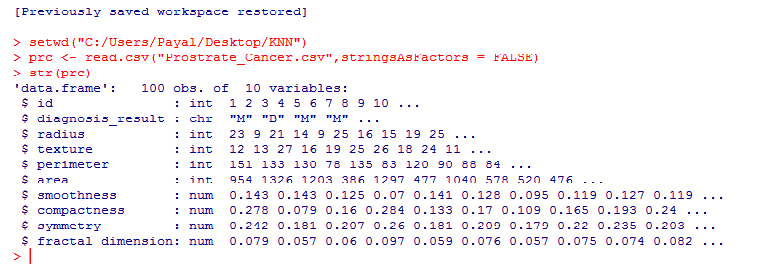
setwd("C:/Users/Payal/Desktop/KNN") #Using this command, we've imported the ‘Prostate_Cancer.csv’ data file. This command is used to point to the folder containing the required file. Do keep in mind, that it’s a common mistake to use “\” instead of “/” after the setwd command.
prc <- read.csv("Prostate_Cancer.csv",stringsAsFactors = FALSE) #This command imports the required data set and saves it to the prc data frame.
stringsAsFactors = FALSE #This command helps to convert every character vector to a factor wherever it makes sense.
str(prc) #We use this command to see whether the data is structured or not.
We find that the data is structured with 10 variables and 100 observations. If we observe the data set, the first variable ‘id’ is unique in nature and can be removed as it does not provide useful information.
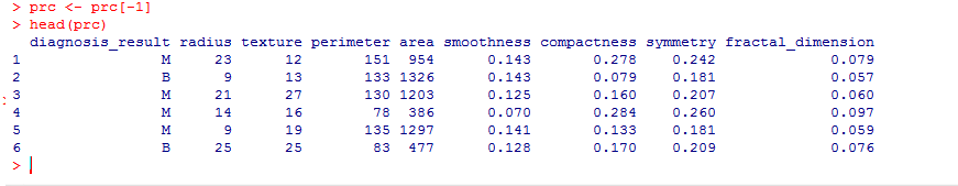
prc <- prc[-1] #removes the first variable(id) from the data set.
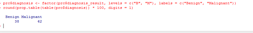
The data set contains patients who have been diagnosed with either Malignant (M) or Benign (B) cancer
table(prc$diagnosis_result) # it helps us to get the numbers of patients
(The variable diagnosis_result is our target variable i.e. this variable will determine the results of the diagnosis based on the 8 numeric variables)
In case we wish to rename B as”Benign” and M as “Malignant” and see the results in the percentage form, we may write as:
prc$diagnosis <- factor(prc$diagnosis_result, levels = c("B", "M"), labels = c("Benign", "Malignant"))
round(prop.table(table(prc$diagnosis)) * 100, digits = 1) # it gives the result in the percentage form rounded of to 1 decimal place( and so it’s digits = 1)
Normalizing numeric data
This feature is of paramount importance since the scale used for the values for each variable might be different. The best practice is to normalize the data and transform all the values to a common scale.
normalize <- function(x) {
return ((x - min(x)) / (max(x) - min(x))) }
Once we run this code, we are required to normalize the numeric features in the data set. Instead of normalizing each of the 8 individual variables we use:
prc_n <- as.data.frame(lapply(prc[2:9], normalize))
The first variable in our data set (after removal of id) is ‘diagnosis_result’ which is not numeric in nature. So, we start from 2nd variable. The function lapply() applies normalize() to each feature in the data frame. The final result is stored to prc_n data frame using as.data.frame() function
Let’s check using the variable ‘radius’ whether the data has been normalized.
summary(prc_n$radius)
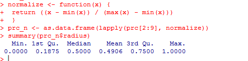
The results show that the data has been normalized. Do try with the other variables such as perimeter, area etc.
Creating training and test data set
The kNN algorithm is applied to the training data set and the results are verified on the test data set.
For this, we would divide the data set into 2 portions in the ratio of 65: 35 (assumed) for the training and test data set respectively. You may use a different ratio altogether depending on the business requirement!
We shall divide the prc_n data frame into prc_train and prc_test data frames
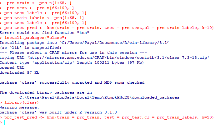
prc_train <- prc_n[1:65,]
prc_test <- prc_n[66:100,]
A blank value in each of the above statements indicate that all rows and columns should be included.
Our target variable is ‘diagnosis_result’ which we have not included in our training and test data sets.
prc_train_labels <- prc[1:65, 1]
prc_test_labels <- prc[66:100, 1]   #This code takes the diagnosis factor in column 1 of the prc data frame and on turn creates prc_train_labels and prc_test_labels data frame.
Step 3 – Training a model on data
The knn () function needs to be used to train a model for which we need to install a package ‘class’. The knn() function identifies the k-nearest neighbors using Euclidean distance where k is a user-specified number.
You need to type in the following commands to use knn()
install.packages(“class”)
library(class)
Now we are ready to use the knn() function to classify test data
prc_test_pred <- knn(train = prc_train, test = prc_test,cl = prc_train_labels, k=10)
The value for k is generally chosen as the square root of the number of observations.
knn() returns a factor value of predicted labels for each of the examples in the test data set which is then assigned to the data frame prc_test_pred
Step 4 – Evaluate the model performance
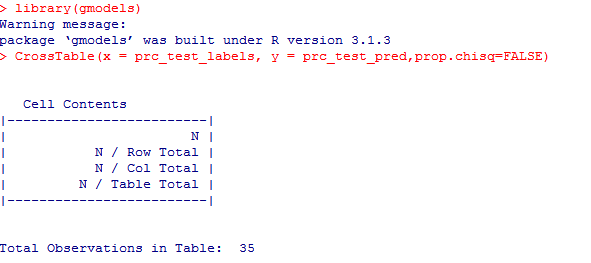
We have built the model but we also need to check the accuracy of the predicted values in prc_test_pred as to whether they match up with the known values in prc_test_labels. To ensure this, we need to use the CrossTable() function available in the package ‘gmodels’.
We can install it using:
install.packages("gmodels")
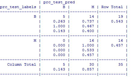
The test data consisted of 35 observations. Out of which 5 cases have been accurately predicted (TN->True Negatives) as Benign (B) in nature which constitutes 14.3%. Also, 16 out of 35 observations were accurately predicted (TP-> True Positives) as Malignant (M) in nature which constitutes 45.7%. Thus a total of 16 out of 35 predictions where TP i.e, True Positive in nature.
There were no cases of False Negatives (FN) meaning no cases were recorded which actually are malignant in nature but got predicted as benign. The FN’s if any poses a potential threat for the same reason and the main focus to increase the accuracy of the model is to reduce FN’s.
There were 14 cases of False Positives (FP) meaning 14 cases were actually benign in nature but got predicted as malignant.
The total accuracy of the model is 60 %( (TN+TP)/35) which shows that there may be chances to improve the model performance
Step 5 – Improve the performance of the model
This can be taken into account by repeating the steps 3 and 4 and by changing the k-value. Generally, it is the square root of the observations and in this case we took k=10 which is a perfect square root of 100.The k-value may be fluctuated in and around the value of 10 to check the increased accuracy of the model. Do try it out with values of your choice to increase the accuracy! Also remember, to keep the value of FN’s as low as possible.
End Notes
For practice purpose, you can also solicit a dummy data set and execute the above mentioned codes to get a taste of the kNN algorithm. The results may not be that precise taking into account the nature of data but one thing for sure: the ability to understand the CrossTable() function and to interpret the results is what we should achieve.
In this article, I’ve explained kNN algorithm using an interesting example and a case study where I have demonstrated the process to apply kNN algorithm in building models.
Did you find this article helpful? Please share your opinions / thoughts in the comments section below.

This article was originally written by Payel Roy Choudhury, before Kunal did his experiment to set the tone. Payel has completed her MBA with specialization in Analytics from Narsee Monjee Institute of Management Studies (NMIMS) and is currently working with ZS Associates. She is looking forward to contribute regularly to Analytics Vidhya.


Hi, Just a question, how do we know that there is a need to normalize data ? i.e. "This feature is of paramount importance since the scale used for the values for each variable might be different. The best practice is to normalize the data and transform all the values to a common scale." Can you explain this? Thanks!
Hi , usually the algorithm use euclidian distance , therefore you have to normalize data because feature like "area" is in range (400 - 1200) and features like symmetry has value between 0.1 - 0.2 , hence simmetry will have small importance in your model and "area" will decide your entire model. This is difference in range is useful only when you wanna give more importance to a certain feature. sorry bad english ;D
This is a great knowledge share. However I am not able to access the initial data set. Is it possible to share the data set through link or mail so that I can try KNN in R?
excellent article!!!!!