Building Trust in Machine Learning Models (using LIME in Python)
The value is not in software, the value is in data, and this is really important for every single company, that they understand what data they’ve got.
-John Straw
Introduction
More and more companies are now aware of the power of data. Machine Learning models are increasing in popularity and are now being used to solve a wide variety of business problems using data. Having said that, it is also true that there is always a trade-off between accuracy of models & its interpretability.
In general, if accuracy has to be improved, data scientists have to resort to using complicated algorithms like Bagging, Boosting, Random Forests etc. which are “Blackbox” methods. It is no wonder that many of the winning entries in Kaggle or Analytics Vidhya competitions tend to use algorithms like XGBoost, where there is no requirement to explain the process of generating the predictions to a business user. On the other hand, in a business setting, simpler models that are more interpretable like Linear Regression, Logistic Regression, Decision Trees, etc. are used even if the predictions are less accurate.
This situation has got to change – the trade-off between accuracy & interpretability is not acceptable. We need to find ways to use powerful black-box algorithms even in a business setting and still be able to explain the logic behind the predictions intuitively to a business user. With increased trust in predictions, organisations will deploy machine learning models more extensively within the enterprise. The question is – “How do we build trust in Machine Learning Models”?
Table of Contents
- Motivation
- The Problem
2.1 Steps for model building
2.2 LIME steps to make your models more interpretable - End Notes
1. Motivation
It is in this context, I find the paper titled “Why Should I Trust You?”- Explaining the Predictions of Any Classifier [1] intriguing & interesting. In this paper [1] , the authors explain a framework called LIME (Locally Interpretable Model-Agnostic Explanations), which is an algorithm that can explain the predictions of any classifier or regressor in a faithful way, by approximating it locally with an interpretable model. In the paper, there are many examples of problems where the predictions from black-box algorithms (even as extreme as Deep Learning) can be formulated in an interpretable fashion. I am not going to explain the paper in this blog but rather show how it can be implemented in our own classification problems.
2. The Problem
Sigma Cab’s Surge Pricing Type Classification
In February this year, Analytics Vidhya ran a machine learning competition in which the objective was to predict the “Surge Pricing Type” for Sigma Cab – a taxi aggregation service. This was a multiclass classification problem. In this blog, we will see how to make predictions for this dataset and use LIME to make the predictions interpretable. The intent here is not to build the best possible model but rather the focus is on the aspect of interpretability.
2.1 Steps for Model Building
# Step 1 – Import all libraries
# Step 2 – Define Functions, variables and dictionaries
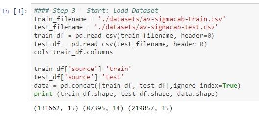
# Step 3 – Load Training dataset
# Step 4 – Understand the data (Descriptive Statistics, Visualization)
# Step 5 – Data Pre-processing (Handle Missing data & outliers, Feature Engineering, Feature Transformation etc.)
# Step 6 – Feature Selection
# Step 7 – Create the validation set
# Step 8 – Compare Algorithms to find candidate algorithms?
# Step 9 – Algorithm(s) Tuning
# Step 10 – Finalize Model(s)
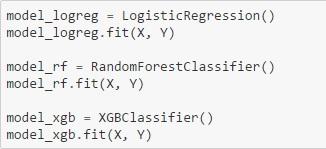
In this case, we are fitting 3 models on the training data so that we can compare the explanations provided. The 3 models are a) Logistic Regression, b) Random Forests, c) XGBoost.
2.2 Steps for using Lime to make your model interpretable
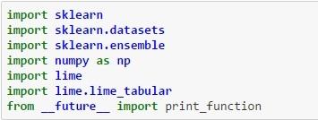
LIME Step 1 – After installing LIME (On ANACONDA distribution – pip install LIME), import the relevant libraries as shown below:
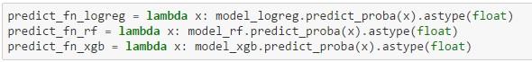
LIME Step 2 – Create a lambda function for each classifier that will return the predicted probability for the target variable (surge pricing type) given the set of features
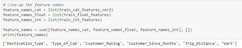
LIME Step 3 – Create a concatenated list of all feature names which will be utilised by the LIME explainer in subsequent steps
LIME Step 4 – This is the ‘magical’ step that creates the explainer

The parameters used by the function are:
- X_train = Training set
- feature_names = Concatenated list of all feature names
- class_names = Target values
- categorical_features = List of categorical columns in the dataset
- categorical_names = List of the categorical column names
- Kernel width = Parameter to control the linearity of the induced model; the larger the width more linear is the model
LIME Step 5 – Obtain the explanations from LIME for particular values in the validation dataset
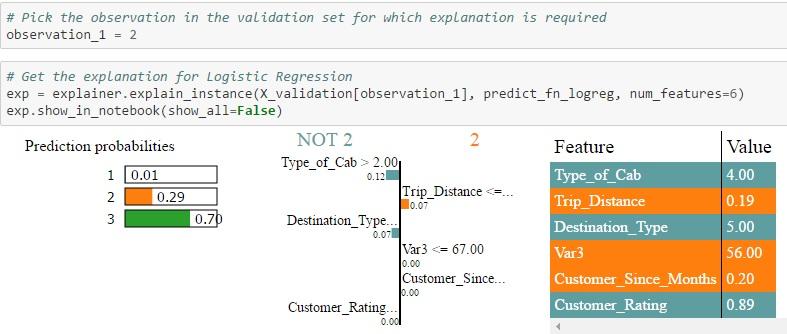
Pick particular observations in the validation dataset to get their probability values for each class. LIME will provide an explanation as to the reason for assigning the probability. Compare the probability values to the actual class of the target variable for that prediction.
Output is shown for 2 observations:
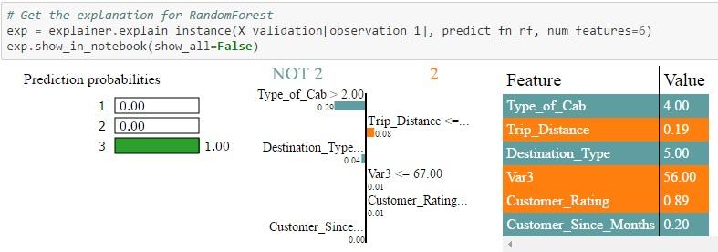
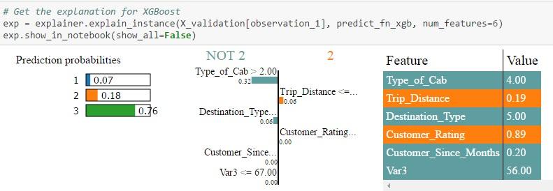
- Id = 2 in validation set: All three algorithms assign a higher probability to type 3 which is the actual value. But the probability ranges from 0.7 to 1.0 with Random Forest assigning the maximum probability. Also, you can see that the weight assigned by the different algorithms to each feature are quite different. Also, when you look at the NOT 2 | 2 table, you can see the weights assigned by different algorithms to each feature. For example, Type of Cab > 2 is assigned a weight of 0.12 in the case of Logistic Regression, a weight of 0.29 in the case of Random Forest and 0.32 in the case of Xgboost. Each feature is then color-coded to indicate whether it is contributing to the prediction of 2 (Orange) or NOT 2 (Grey) in the feature-value-table. The Feature-Value table by itself shows the actual values of the features for that particular record (in this case Id = 2)
(Note: The visualisation is not powerful enough to show the feature weights for all classes in a multi-class scenario but the same process is applicable to differentiate between class 1 & 3 also)
2. Id = 45 in validation set: In this case, only Random Forest is able to assign a higher probability to type 1 which is the actual value. Both Logistic Regression & XGBoost predicts that type 2 has a higher probability. Also, when you look at the NOT 2 | 2 table, you can see the weights assigned by different algorithms to each feature. For example, Trip Distance > 0.35 is assigned a weight of 0.01 in the case of Logistic Regression, a weight of 0.02 in the case of Random Forest and 0.01 in the case of Xgboost. Each feature is then color-coded to indicate whether it is contributing to the prediction of 2 (Orange) or NOT 2 (Grey) in the feature-value-table. The Feature-Value table by itself shows the actual values of the features for that particular record (in this case Id = 45)
(Note: The visualisation is not powerful enough to show the feature weights for all classes in a multi-class scenario but the same process is applicable to differentiate between class 1 & 3 also)
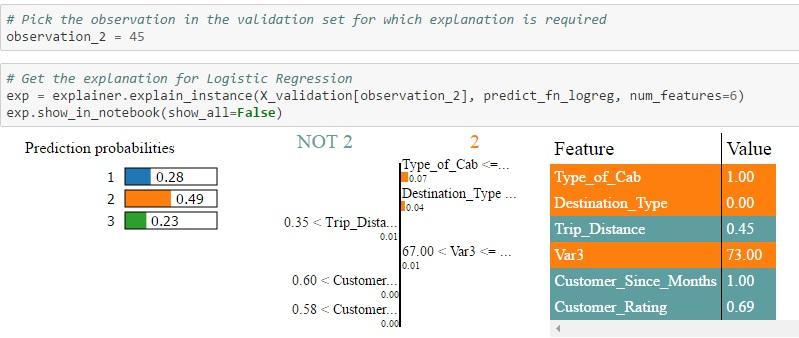
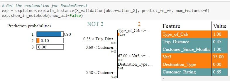
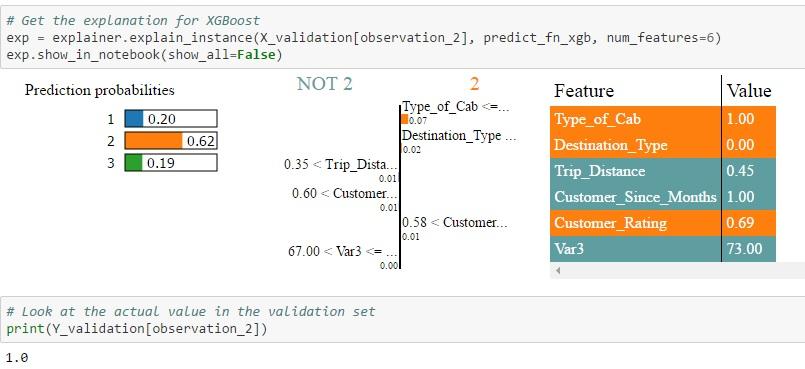
The probability values for each class is different for each algorithm as the feature weights computed by each algorithm are different. Depending on the actual value of the features for a particular record and the weights assigned to those features, the algorithm computes the class probability and then predicts the class having the highest probability. These results can be interpreted by a subject matter expert to see which algorithm is picking up the right signals / features to make the prediction. Essentially, the black box algorithms have become white box in the sense that now we know what drives the algorithms to make its predictions.
Here’s the whole code for your reference
# Load All Libraries
import pandas as pd
import numpy as np
import matplotlib.pyplot as plt
import seaborn as sns
from sklearn.base import TransformerMixin
from sklearn.preprocessing import Imputer
from sklearn.preprocessing import MinMaxScaler
from sklearn.preprocessing import LabelEncoder
from sklearn.metrics import accuracy_score
from sklearn import cross_validation
from sklearn.linear_model import LogisticRegression
from sklearn.ensemble import RandomForestClassifier
from xgboost import XGBClassifier
#### Write your functions and define variables
def num_missing(x):
return sum(x.isnull())
class DataFrameImputer(TransformerMixin):
def __init__(self):
"""Impute missing values.
Columns of dtype object are imputed with the most frequent value
in column.
Columns of other types are imputed with mean of column.
"""
def fit(self, X, y=None):
self.fill = pd.Series([X[c].value_counts().index[0]
if X[c].dtype == np.dtype('O') else X[c].mean() for c in X],
index=X.columns)
return self
def transform(self, X, y=None):
return X.fillna(self.fill)
#### Load Dataset
train_filename = './datasets/av-sigmacab-train.csv'
test_filename = './datasets/av-sigmacab-test.csv'
train_df = pd.read_csv(train_filename, header=0)
test_df = pd.read_csv(test_filename, header=0)
cols=train_df.columns
train_df['source']='train'
test_df['source']='test'
data = pd.concat([train_df, test_df],ignore_index=True)
print (train_df.shape, test_df.shape, data.shape)
# Handling missing values
imputer_mean = Imputer(missing_values = 'NaN', strategy = 'mean', axis = 0)
imputer_median = Imputer(missing_values = 'NaN', strategy = 'median', axis = 0)
imputer_mode = Imputer(missing_values = 'NaN', strategy = 'most_frequent', axis = 0)
data["Life_Style_Index"]=imputer_mean.fit_transform(data[["Life_Style_Index"]]).ravel()
data["Var1"]=imputer_mean.fit_transform(data[["Var1"]]).ravel()
data["Customer_Since_Months"]=imputer_median.fit_transform(data[["Customer_Since_Months"]]).ravel()
X = pd.DataFrame(data)
data = DataFrameImputer().fit_transform(X)
print (data.apply(num_missing, axis=0))
#Divide into test and train:
train_df = data.loc[data['source']=="train"]
test_df = data.loc[data['source']=="test"]
# Drop unwanted columns
train_df = train_df.drop(['Trip_ID','Cancellation_Last_1Month','Confidence_Life_Style_Index','Gender','Life_Style_Index','Var1','Var2','source',],axis=1)
#### Extract the label column
train_target = np.ravel(np.array(train_df['Surge_Pricing_Type'].values))
train_df = train_df.drop(['Surge_Pricing_Type'],axis=1)
# Extract features
float_columns=[]
cat_columns=[]
int_columns=[]
for i in train_df.columns:
if train_df[i].dtype == 'float' :
float_columns.append(i)
elif train_df[i].dtype == 'int64':
int_columns.append(i)
elif train_df[i].dtype == 'object':
cat_columns.append(i)
train_cat_features = train_df[cat_columns]
train_float_features = train_df[float_columns]
train_int_features = train_df[int_columns]
## Transformation of categorical columns
# Label Encoding:
#train_cat_features_ver2 = pd.get_dummies(train_cat_features, columns=['Destination_Type','Type_of_Cab'])
train_cat_features_ver2 = train_cat_features.apply(LabelEncoder().fit_transform)
## Transformation of float columns
# Rescale data (between 0 and 1)
scaler = MinMaxScaler(feature_range=(0, 1))
for i in train_float_features.columns:
X_temp = train_float_features[i].reshape(-1,1)
train_float_features[i] = scaler.fit_transform(X_temp)
#### Finalize X & Y
temp_1 = np.concatenate((train_cat_features_ver2,train_float_features),axis=1)
train_transformed_features = np.concatenate((temp_1,train_int_features),axis=1)
train_transformed_features = pd.DataFrame(data=train_transformed_features)
array = train_transformed_features.values
number_of_features = len(array[0])
X = array[:,0:number_of_features]
Y = train_target
# Split into training and validation set
validation_size = 0.2
seed = 7
X_train, X_validation, Y_train, Y_validation = cross_validation.train_test_split(X, Y, test_size=validation_size, random_state=seed)
scoring = 'accuracy'
# Model 1 - Logisitic Regression
model_logreg = LogisticRegression()
model_logreg.fit(X_train, Y_train)
accuracy_score(Y_validation, model_logreg.predict(X_validation))
# Model 2 - RandomForest Classifier
model_rf = RandomForestClassifier()
model_rf.fit(X_train, Y_train)
accuracy_score(Y_validation, model_rf.predict(X_validation))
# Model 3 - XGB Classifier
model_xgb = XGBClassifier()
model_xgb.fit(X_train, Y_train)
accuracy_score(Y_validation, model_xgb.predict(X_validation))
model_logreg = LogisticRegression()
model_logreg.fit(X, Y)
model_rf = RandomForestClassifier()
model_rf.fit(X, Y)
model_xgb = XGBClassifier()
model_xgb.fit(X, Y)
# LIME SECTION
import sklearn
import sklearn.datasets
import sklearn.ensemble
import numpy as np
import lime
import lime.lime_tabular
from __future__ import print_function
predict_fn_logreg = lambda x: model_logreg.predict_proba(x).astype(float)
predict_fn_rf = lambda x: model_rf.predict_proba(x).astype(float)
predict_fn_xgb = lambda x: model_xgb.predict_proba(x).astype(float)
# Line-up the feature names
feature_names_cat = list(train_cat_features_ver2)
feature_names_float = list(train_float_features)
feature_names_int = list(train_int_features)
feature_names = sum([feature_names_cat, feature_names_float, feature_names_int], [])
print(feature_names)
# Create the LIME Explainer
explainer = lime.lime_tabular.LimeTabularExplainer(X_train ,feature_names = feature_names,class_names=['1','2','3'],
categorical_features=cat_columns,
categorical_names=feature_names_cat, kernel_width=3)
# Pick the observation in the validation set for which explanation is required
observation_1 = 2
# Get the explanation for Logistic Regression
exp = explainer.explain_instance(X_validation[observation_1], predict_fn_logreg, num_features=6)
exp.show_in_notebook(show_all=False)
# Get the explanation for RandomForest
exp = explainer.explain_instance(X_validation[observation_1], predict_fn_rf, num_features=6)
exp.show_in_notebook(show_all=False)
# Get the explanation for XGBoost
exp = explainer.explain_instance(X_validation[observation_1], predict_fn_xgb, num_features=6)
exp.show_in_notebook(show_all=False)
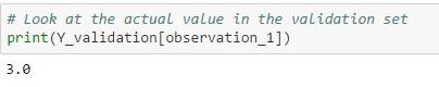
# Look at the actual value in the validation set
print(Y_validation[observation_1])
# Pick the observation in the validation set for which explanation is required
observation_2 = 45
# Get the explanation for Logistic Regression
exp = explainer.explain_instance(X_validation[observation_2], predict_fn_logreg, num_features=6)
exp.show_in_notebook(show_all=False)
# Get the explanation for RandomForest
exp = explainer.explain_instance(X_validation[observation_2], predict_fn_rf, num_features=6)
exp.show_in_notebook(show_all=False)
# Get the explanation for XGBoost
exp = explainer.explain_instance(X_validation[observation_2], predict_fn_xgb, num_features=6)
exp.show_in_notebook(show_all=False)
# Look at the actual value in the validation set
print(Y_validation[observation_2])
3. End Notes
I hope you are as excited as me after looking at these results. The output of LIME provides an intuition into the inner workings of machine learning algorithms as to the features that are being used to arrive at a prediction. If LIME or similar algorithms can help in providing interpretable output for any type of blackbox algorithm, it will go a long way in getting the buy-in from business users to trust the output of machine learning algorithms. By building such trust, powerful methods can be deployed in a business context achieving the twin benefits of higher accuracy and interpretability. Please do check out the LIME paper for the math behind this fascinating development.
References
[1] Marco Tulio Ribeiro, Sameer Singh, Carlos Guestrin. “Why Should I Trust You?” Explaining the Predictions of Any Classifier. Proceedings of the 22nd ACM SIGKDD International Conference on Knowledge Discovery and Data Mining
 Karthikeyan Sankaran is currently a Director at LatentView Analytics which provides solutions at the intersection of Business, Technology & Math to business problems across a wide range of industries. Karthik has close to two decades of experience in the Information Technology industry having worked in multiple roles across the space of Data Management, Business Intelligence & Analytics.
This story was received as part of “The Mightiest Pen” contest on Analytics Vidhya. Karthikeyan’s entry was one of the winning entries in the competition.


Very Informative and well explained.
useful and well described
Great! Is it possible to do something similar with R?
Thanks @Preeti, @shiva, @ Bernardo. @Bernardo - To my knowledge, this is possible only in Python for now. Am not aware of LIME equivalent packages in R. Will investigate and let you know.
This looks great ! Thanks for sharing. Am very interested to see how it works with a deep learning model. Though one concern I see is that if explanation were to differ from observation to observation, will that really be a consolation to the business and make it a "white box". Nevertheless a great milestone.
Great articles @Karthikeyan. I m really inspired by your story of becoming data science hacker from delivery head. I have couple of questions for you : 1. have you written all above code your self ? 2. What kind of work you do as part of your new job as director. ? Is it only discussion with teams or you do coding ( data cleaning , model tuning , trying different models etc )
very useful for the domain people who need s interpret the numbers
Is the dataset available somewhere? It is no longer on the minihack page. Would be incredibly helpful if you could post a link
Hi Karthikeyan, I am a big fan of your posts. Just one quick question, at the time of creating the explainer I get the following error: TypeError: unhashable type: 'slice'. @Karthikeyan by any chance do you happen to know what I am doing wrong?
Hi, Can you please provide the link to download the dataset mentioned in this article for practice Thanks, Ram