Introduction
Neural network is an information-processing machine and can be viewed as analogous to human nervous system. Just like human nervous system, which is made up of interconnected neurons, a neural network is made up of interconnected information processing units. The information processing units do not work in a linear manner. In fact, neural network draws its strength from parallel processing of information, which allows it to deal with non-linearity. Neural network becomes handy to infer meaning and detect patterns from complex data sets.

Neural network is considered as one of the most useful technique in the world of data analytics. However, it is complex and is often regarded as a black box, i.e. users view the input and output of a neural network but remain clueless about the knowledge generating process. We hope that the article will help readers learn about the internal mechanism of a neural network and get hands-on experience to implement it in R.
Table of contents
The Basics of Neural Network
A neural network is a model characterized by an activation function, which is used by interconnected information processing units to transform input into output. A neural network has always been compared to human nervous system. Information in passed through interconnected units analogous to information passage through neurons in humans. The first layer of the neural network receives the raw input, processes it and passes the processed information to the hidden layers. The hidden layer passes the information to the last layer, which produces the output. The advantage of neural network is that it is adaptive in nature. It learns from the information provided, i.e. trains itself from the data, which has a known outcome and optimizes its weights for a better prediction in situations with unknown outcome.
A perceptron, viz. single layer neural network, is the most basic form of a neural network. A perceptron receives multidimensional input and processes it using a weighted summation and an activation function. It is trained using a labeled data and learning algorithm that optimize the weights in the summation processor. A major limitation of perceptron model is its inability to deal with non-linearity. A multilayered neural network overcomes this limitation and helps solve non-linear problems. The input layer connects with hidden layer, which in turn connects to the output layer. The connections are weighted and weights are optimized using a learning rule.
There are many learning rules that are used with neural network:
a) least mean square;
b) gradient descent;
c) newton’s rule;
d) conjugate gradient etc.
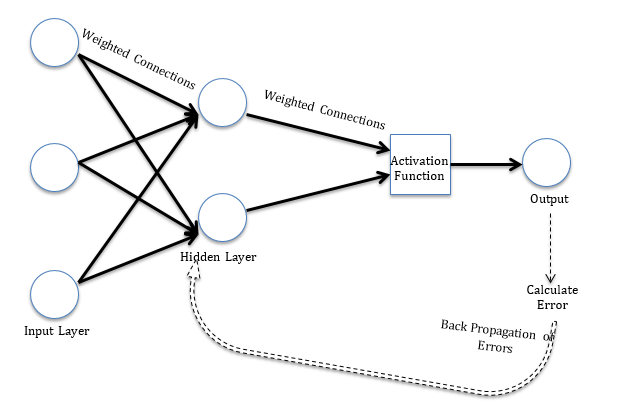
The learning rules can be used in conjunction with backpropgation error method. The learning rule is used to calculate the error at the output unit. This error is backpropagated to all the units such that the error at each unit is proportional to the contribution of that unit towards total error at the output unit. The errors at each unit are then used to optimize the weight at each connection. Figure 1 displays the structure of a simple neural network model for better understanding.
Types of Neural Network in R
In R, you can implement various types of neural networks using different packages. Here are some common types:
Feedforward Neural Networks (FFNN):
Implemented in packages like nnet, neuralnet, and caret. Suitable for tasks like classification and regression.
Convolutional Neural Networks (CNN):
Implemented in packages like keras, tensorflow, and torch. Ideal for image recognition, computer vision, and natural language processing tasks where spatial relationships matter.
Recurrent Neural Networks (RNN):
Implemented in packages like keras, tensorflow, and torch. Suitable for sequential data tasks such as time series analysis, text generation, and speech recognition.
Long Short-Term Memory Networks (LSTM):
A type of RNN designed to overcome the vanishing gradient problem. Implemented in packages like keras, tensorflow, and torch.
Gated Recurrent Unit Networks (GRU):
Similar to LSTM but with a simpler architecture. Also implemented in packages like keras, tensorflow, and torch. Autoencoders:
Implemented in packages like keras, h2o, and deepnet. Used for unsupervised learning, dimensionality reduction, and anomaly detection tasks.
Generative Adversarial Networks (GAN):
Implemented in packages like keras and torch. Used for generating synthetic data, image translation, and data augmentation.
Deep Belief Networks (DBN):
Implemented in packages like deepnet, RBM, and h2o. Used for feature learning, pre-training deep architectures, and unsupervised learning. These are just a few examples, and there are many other specialized architectures and variations available in R through various packages. Choose the one that best suits your problem domain and data characteristics. When using these packages, consider aspects such as training data, loss function, data preparation, and cross entropy for optimal performance.
Implementation of Neural Network in R
Implementing neural networks in R can be done using various packages, but one of the most commonly used ones is neuralnet. This package provides functions to create, train, and evaluate neural networks. Below is a simple example of implementing a neural network for a classification task using neuralnet:
# Install and load the neuralnet package
install.packages("neuralnet")
library(neuralnet)

# Generate some sample data
set.seed(123)
data <- data.frame(
  x1 = rnorm(100),
  x2 = rnorm(100),
  class = factor(sample(0:1, 100, replace = TRUE))
)

# Train-test split
train_indices <- sample(1:nrow(data), 0.7 * nrow(data))
train_data <- data[train_indices, ]
test_data <- data[-train_indices, ]

# Define and train the neural network
nn <- neuralnet(class ~ x1 + x2, data = train_data, hidden = 5)

# Make predictions on test data
predicted <- round(predict(nn, test_data))

# Evaluate the model
confusion_matrix <- table(predicted, test_data$class)
accuracy <- sum(diag(confusion_matrix)) / sum(confusion_matrix)
print(confusion_matrix)
print(paste("Accuracy:", accuracy))
This code first installs and loads the neuralnet package. Then it generates some sample data for a classification problem. After splitting the data into training and testing sets, it defines a neural network with one hidden layer of 5 neurons and trains it using the training data. Finally, it evaluates the trained model using the test data by computing a confusion matrix and accuracy.
You can further tune the neural network architecture, such as the number of hidden layers, number of neurons in each layer, activation functions, etc., according to your specific problem and requirements.
Fitting Neural Network in R
Now we will fit a neural network model in R. In this article, we use a subset of cereal dataset shared by Carnegie Mellon University (CMU). The details of the dataset are on the following link: http://lib.stat.cmu.edu/DASL/Datafiles/Cereals.html. The objective is to predict rating of the cereals variables such as calories, proteins, fat etc. The R script is provided side by side and is commented for better understanding of the user. . The data is in .csv format and can be downloaded by clicking: cereals.
Please set working directory in R using setwd( ) function, and keep cereal.csv in the working directory. We use rating as the dependent variable and calories, proteins, fat, sodium and fiber as the independent variables. We divide the data into training and test set. Training set is used to find the relationship between dependent and independent variables while the test set assesses the performance of the model. We use 60% of the dataset as training set. The assignment of the data to training and test set is done using random sampling. We perform random sampling on R using sample ( ) function. We have used set.seed( ) to generate same random sample everytime and maintain consistency. We will use the index variable while fitting neural network to create training and test data sets. The R script is as follows:
## Creating index variable

# Read the Data
data = read.csv("cereals.csv", header=T)

# Random sampling
samplesize = 0.60 * nrow(data)
set.seed(80)
index = sample( seq_len ( nrow ( data ) ), size = samplesize )

# Create training and test set
datatrain = data[ index, ]
datatest = data[ -index, ]
Now we fit a neural network on our data. We use neuralnet library for the analysis. The first step is to scale the cereal dataset. The scaling of data is essential because otherwise a variable may have large impact on the prediction variable only because of its scale. Using unscaled may lead to meaningless results. The common techniques to scale data are: min-max normalization, Z-score normalization, median and MAD, and tan-h estimators. The min-max normalization transforms the data into a common range, thus removing the scaling effect from all the variables. Unlike Z-score normalization and median and MAD method, the min-max method retains the original distribution of the variables. We use min-max normalization to scale the data. The R script for scaling the data is as follows.
## Scale data for neural network

max = apply(data , 2 , max)
min = apply(data, 2 , min)
scaled = as.data.frame(scale(data, center = min, scale = max - min))
The scaled data is used to fit the neural network. We visualize the neural network with weights for each of the variable. The R script is as follows.
## Fit neural network

# install library
install.packages("neuralnet ")

# load library
library(neuralnet)

# creating training and test set
trainNN = scaled[index , ]
testNN = scaled[-index , ]

# fit neural network
set.seed(2)
NN = neuralnet(rating ~ calories + protein + fat + sodium + fiber, trainNN, hidden = 3 , linear.output = T )

# plot neural network
plot(NN)
Figure 3 visualizes the computed neural network. Our model has 3 neurons in its hidden layer. The black lines show the connections with weights. The weights are calculated using the back propagation algorithm explained earlier. The blue line is the displays the bias term.
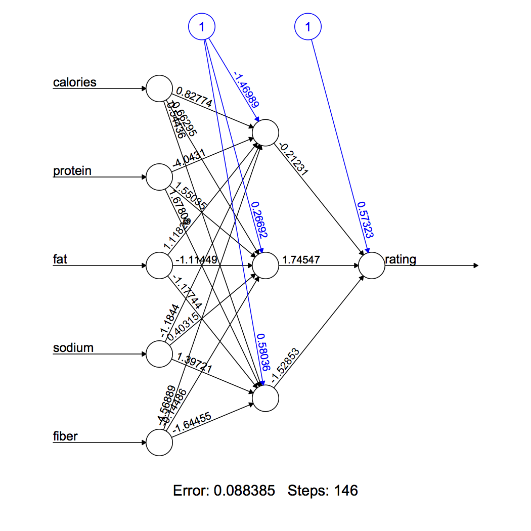
Figure 2 Neural Network
We predict the rating using the neural network model. The reader must remember that the predicted rating will be scaled and it must me transformed in order to make a comparison with real rating. We also compare the predicted rating with real rating using visualization. The RMSE for neural network model is 6.05. The reader can learn more about RMSE in another article, which can be accessed by clicking here. The R script is as follows:
## Prediction using neural network

predict_testNN = compute(NN, testNN[,c(1:5)])
predict_testNN = (predict_testNN$net.result * (max(data$rating) - min(data$rating))) + min(data$rating)

plot(datatest$rating, predict_testNN, col='blue', pch=16, ylab = "predicted rating NN", xlab = "real rating")

abline(0,1)

# Calculate Root Mean Square Error (RMSE)
RMSE.NN = (sum((datatest$rating - predict_testNN)^2) / nrow(datatest)) ^ 0.5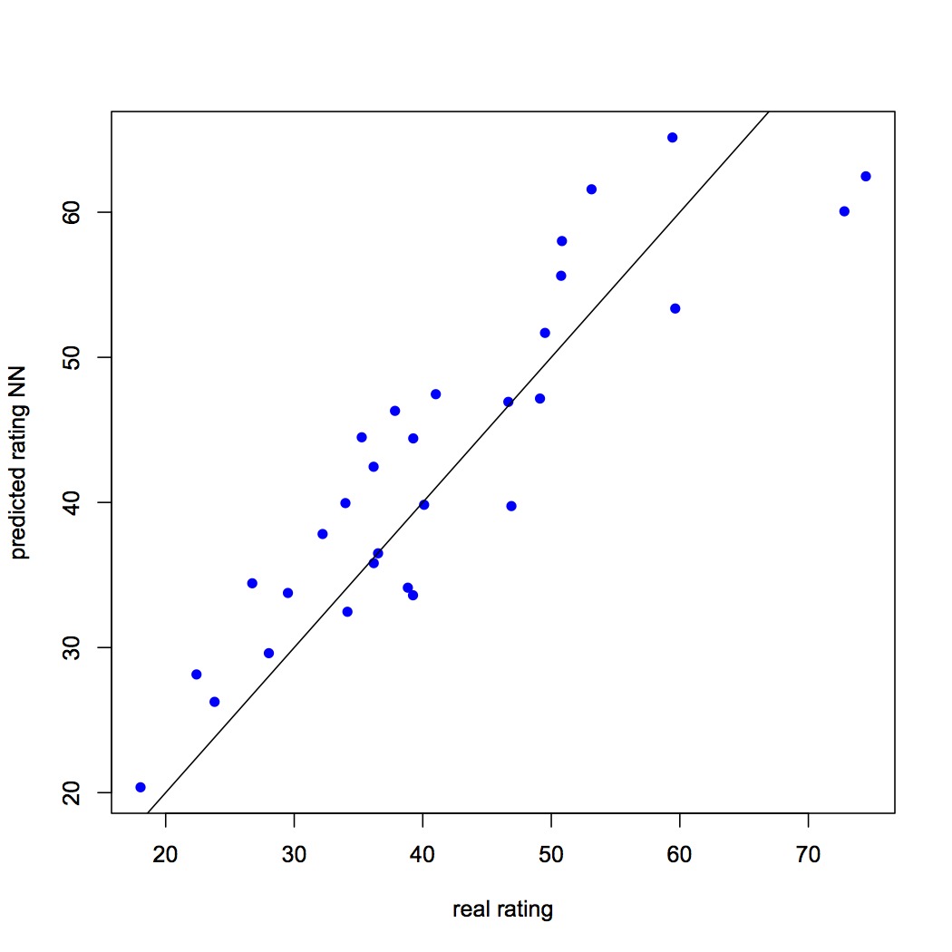
Figure 3: Predicted rating vs. real rating using neural network
Cross Validation of a Neural Network
We have evaluated our neural network method using RMSE, which is a residual method of evaluation. The major problem of residual evaluation methods is that it does not inform us about the behaviour of our model when new data is introduced. We tried to deal with the “new data” problem by splitting our data into training and test set, constructing the model on training set and evaluating the model by calculating RMSE for the test set. The training-test split was nothing but the simplest form of cross validation method known as holdout method. A limitation of the holdout method is the variance of performance evaluation metric, in our case RMSE, can be high based on the elements assigned to training and test set.
The second commonly cross validation technique is k-fold cross validation. This method can be viewed as a recurring holdout method. The complete data is partitioned into k equal subsets and each time a subset is assigned as test set while others are used for training the model. Every data point gets a chance to be in test set and training set, thus this method reduces the dependence of performance on test-training split and reduces the variance of performance metrics. The extreme case of k-fold cross validation will occur when k is equal to number of data points. It would mean that the predictive model is trained over all the data points except one data point, which takes the role of a test set. This method of leaving one data point as test set is known as leave-one-out cross validation.
Now we will perform k-fold cross-validation on the neural network model we built in the previous section. The number of elements in the training set, j, are varied from 10 to 65 and for each j, 100 samples are drawn form the dataset. The rest of the elements in each case are assigned to test set. The model is trained on each of the 5600 training datasets and then tested on the corresponding test sets. We compute RMSE of each of the test set. The RMSE values for each of the set is stored in a Matrix[100 X 56]. This method ensures that our results are free of any sample bias and checks for the robustness of our model. We employ nested for loop. The R script is as follows:
## Cross validation of neural network model

# install relevant libraries
install.packages("boot")
install.packages("plyr")

# Load libraries
library(boot)
library(plyr)

# Initialize variables
set.seed(50)
k = 100
RMSE.NN = NULL

List = list( )

# Fit neural network model within nested for loop
for(j in 10:65){
    for (i in 1:k) {
        index = sample(1:nrow(data),j )

        trainNN = scaled[index,]
        testNN = scaled[-index,]
        datatest = data[-index,]

        NN = neuralnet(rating ~ calories + protein + fat + sodium + fiber, trainNN, hidden = 3, linear.output= T)
        predict_testNN = compute(NN,testNN[,c(1:5)])
        predict_testNN = (predict_testNN$net.result*(max(data$rating)-min(data$rating)))+min(data$rating)

        RMSE.NN [i]<- (sum((datatest$rating - predict_testNN)^2)/nrow(datatest))^0.5
    }
    List[[j]] = RMSE.NN
}

Matrix.RMSE = do.call(cbind, List)
The RMSE values can be accessed using the variable Matrix.RMSE. The size of the matrix is large; therefore we will try to make sense of the data through visualizations. First, we will prepare a boxplot for one of the columns in Matrix.RMSE, where training set has length equal to 65. One can prepare these box plots for each of the training set lengths (10 to 65). The R script is as follows.
## Prepare boxplot
boxplot(Matrix.RMSE[,56], ylab = "RMSE", main = "RMSE BoxPlot (length of traning set = 65)")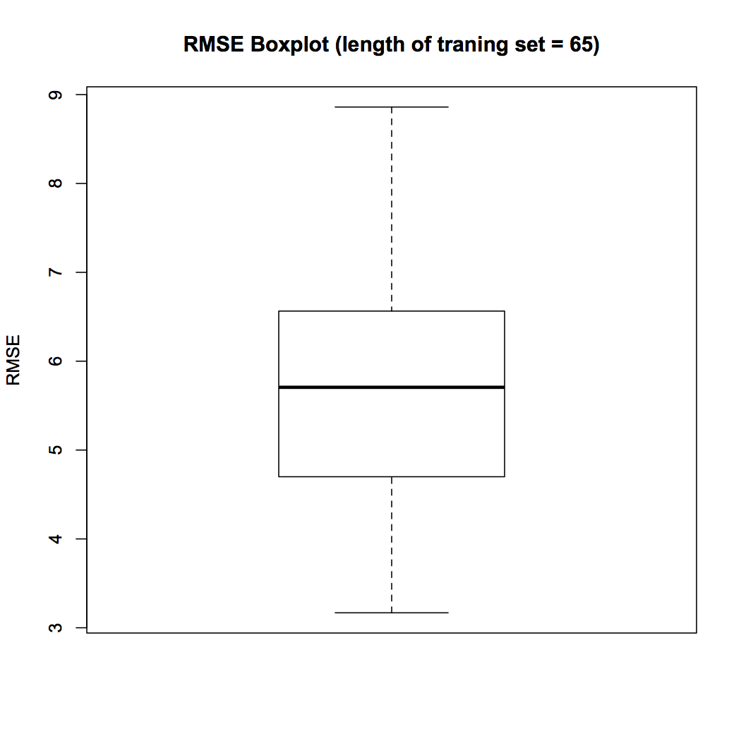
Figure 4 Boxplot
The boxplot in Fig. 4 shows that the median RMSE across 100 samples when length of training set is fixed to 65 is 5.70. In the next visualization we study the variation of RMSE with the length of training set. We calculate the median RMSE for each of the training set length and plot them using the following R script.
## Variation of median RMSE
install.packages("matrixStats")
library(matrixStats)

med = colMedians(Matrix.RMSE)

X = seq(10,65)

plot (med~X, type = "l", xlab = "length of training set", ylab = "median RMSE", main = "Variation of RMSE with length of training set")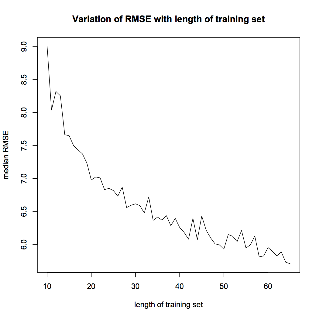
Figure 5 Variation of RMSE
Figure 5 shows that the median RMSE of our model decreases as the length of the training the set. This is an important result. The reader must remember that the model accuracy is dependent on the length of training set. The performance of neural network model is sensitive to training-test split.
Fitting Neural Network in R
Install and Load the Package: First, you need to make sure the neuralnet package is installed. If not, you can install it from CRAN using install.packages(“neuralnet”). Then load the package into your R session
library(neuralnet)Prepare Your Data: Make sure your data is prepared in a format suitable for modeling. This typically involves splitting your data into predictors (features) and the target variable you want to predict.
Train the Neural Network: Use the neuralnet() function to train your neural network model. Specify the formula for the model, the training data, and any other parameters you want to customize. For example:
# Example formula: predict y based on x1 and x2
formula <- y ~ x1 + x2

# Train the neural network
nn <- neuralnet(formula, data = training_data, hidden = c(5, 3))
Make Predictions: Once your model is trained, you can use it to make predictions on new data. Use the predict() function:
predictions <- predict(nn, newdata = test_data)Evaluate the Model: Evaluate the performance of your model using appropriate metrics such as mean squared error, accuracy, etc. This will depend on the nature of your problem (regression, classification, etc.). Utilize these metrics to assess the effectiveness of your deep neural network. For regression tasks, focus on metrics like mean squared error to gauge the disparity between predicted and actual values. Classification tasks may require accuracy or other relevant metrics to measure the model’s classification performance.
Tune Hyperparameters : You can further enhance your model’s performance by tuning hyperparameters such as the number of hidden layers, number of neurons in each layer, learning rate, etc. Experiment with different values and evaluate the impact on model performance. Adjust these hyperparameters within your deep neural network architecture to optimize its efficiency in solving your specific problem. Consider employing techniques such as grid search or random search to systematically explore the hyperparameter space.
Cross-Validation: To ensure your model’s generalization ability, you can perform cross-validation. This involves splitting your data into multiple folds, training the model on different combinations of training and validation sets, and averaging the performance metrics across folds. Cross-validation is particularly beneficial for deep neural networks as it helps mitigate overfitting and provides a more reliable estimate of the model’s performance on unseen data. Implement cross-validation techniques tailored to neural networks, such as k-fold cross-validation, to validate the robustness of your model.
That’s a basic overview of fitting a neural network in R using the Activation Functions neural net package. Feel free to ask if you need further clarification or assistance with any specific step!
End Notes
The article discusses the theoretical aspects of a neural network, its implementation in R and post training evaluation. Neural network is inspired from biological nervous system. Similar to nervous system the information is passed through layers of processors. The significance of variables is represented by weights of each connection. The article provides basic understanding of back propagation algorithm, which is used to assign these weights. In this article we also implement neural network on R. We use a publically available dataset shared by CMU. The aim is to predict the rating of cereals using information such as calories, fat, protein etc. After constructing the neural network we evaluate the model for accuracy and robustness. We compute RMSE and perform cross-validation analysis. In cross validation, we check the variation in model accuracy as the length of training set is changed. We consider training sets with length 10 to 65. For each length a 100 samples are random picked and median RMSE is calculated. We show that model accuracy increases when training set is large. Before using the model for prediction, it is important to check the robustness of performance through cross validation.
The article provides a quick review neural network and is a useful reference for data enthusiasts. We have provided commented R code throughout the article to help readers with hands on experience of using neural networks.
Bio: Chaitanya Sagar is the Founder and CEO of Perceptive Analytics. Perceptive Analytics is one of the top analytics companies in India. It works on Marketing Analytics for ecommerce, Retail and Pharma companies.


Wonderful! Thanks for the excellent learning demo.
Thank you for the post. It is excellent in that you introduce a lot of nuances but explain them and demonstrate them. This is a very high-quality tutorial.
many thanks
Please can you forward the R codes of neural network for time series data forecasting/ prediction
Hi - you can refer this article for a practical implementation
Incorrect- " Figure 3 visualizes the computed neural network. Our model has 3 hidden layers." , should be 3 neurons in 1 hidden layer.
Thanks for the suggestion. We have updated the part
This has been very useful, is there an easy way to alter this code for a binary outcome (e.g. damage (1) or no damage (0)?