Mastering machine learning algorithms isn’t a myth at all. Most beginners start by learning regression. It is simple to learn and use, but does that solve our purpose? Of course not! Because there is a lot more in ML beyond logistic regression and regression problems! For instance, have you heard of support vector regression and support vector machines algorithm or SVM?
Think of machine learning algorithms as an armory packed with axes, swords, blades, bows, daggers, etc. You have various tools, but you ought to learn to use them at the right time. As an analogy, think of ‘Regression’ as a sword capable of slicing and dicing data efficiently but incapable of dealing with highly complex data. That is where ‘Support Vector Machines’ acts like a sharp knife – it works on smaller datasets, but on complex ones, it can be much stronger and more powerful in building machine learning models.
In this article, you will get an understanding of Support Vector Machines (SVM), a widely used algorithm in machine learning. SVM is particularly effective as an SVM classifier, excelling at classification tasks by finding optimal hyperplanes to separate data. We will explore how SVM works and its applications in various domains.
Learning Objectives
“Support Vector Machine” (SVM) is a supervised learning machine learning algorithm that can be used for both classification or regression challenges. However, it is mostly used in classification problems, such as text classification. In the SVM algorithm, we plot each data item as a point in n-dimensional space (where n is the number of features you have), with the value of each feature being the value of a particular coordinate. Then, we perform classification by finding the optimal hyper-plane that differentiates the two classes very well (look at the below snapshot).
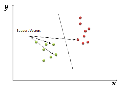
Support Vectors are simply the coordinates of individual observation, and a hyper-plane is a form of SVM visualization. The SVM classifier is a frontier that best segregates the two classes (hyper-plane/line).
Above, we got accustomed to the process of segregating the two classes with a hyper-plane. Now the burning question is, “How can we identify the right hyper-plane?”. Don’t worry; it’s not as hard as you think! Let’s understand:


In the above plot, points to consider are:
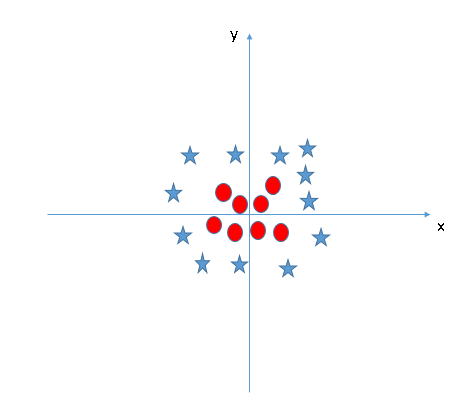
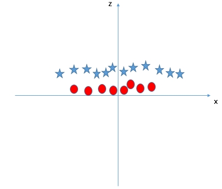
In the SVM classifier, having a linear hyper-plane between these two classes is easy. But, another burning question that arises is if we should we need to add this feature manually to have a hyper-plane. No, the SVM algorithm has a technique called the kernel trick. The SVM kernel transforms low-dimensional input space to a higher dimensional space, making non-separable problems separable, useful for non-linear data separation by applying complex data transformations based on labels.
When we look at the hyper-plane in the original input space, it looks like a circle:

Now, let’s look at the methods to apply the SVM classifier algorithm in a data science challenge.
You can also learn about the working of a Support Vector Machine in data mining video format from this Machine Learning certification course.
In an SVM, a hyperplane is a decision boundary that separates different classes of data points. For instance, in a two-dimensional space, the hyperplane is a line; in a three-dimensional space, it is a plane. The goal of the SVM is to find the optimal hyperplane that maximizes the margin between the classes. The margin is defined as the distance between the hyperplane and the nearest data points from either class.
Support vectors are the data points that are closest to the hyperplane. These points are critical because they determine the position and orientation of the hyperplane. If you remove a support vector, it can change the hyperplane’s position.
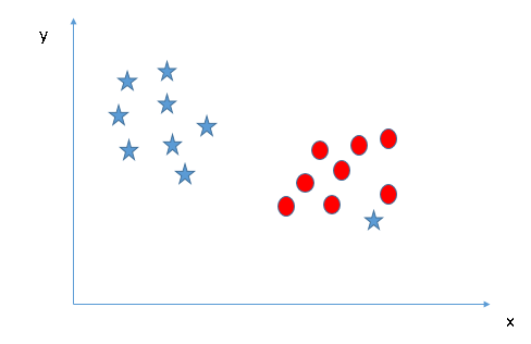
Linear SVM is used when the data is linearly separable, which means that the classes can be separated with a straight line (in 2D) or a flat plane (in 3D). The SVM algorithm finds the hyperplane that best divides the data into classes.
Non-Linear SVM is used when the data is not linearly separable. In such cases, SVM employs kernel functions to transform the data into a higher-dimensional space where a linear separation is possible. The algorithm then finds the optimal hyperplane in this new space.
Kernels are functions that take low-dimensional input space and transform it into a higher-dimensional space. SVM can create complex decision boundaries by using kernel functions. Here are some popular kernel functions:
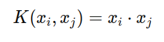
Used when the data is linearly separable.
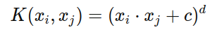
Where c is a constant, and d is the degree of the polynomial. This kernel is useful for classifying data with polynomial relationships.
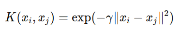
Where γ is a parameter that defines the influence of a single training example. This is one of the most popular kernels for non-linear data.
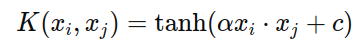
Where α and care kernel parameters. It behaves like a neural network’s activation function.
In Python, scikit-learn is a widely used library for implementing machine learning algorithms. SVM algorithm is also available in the scikit-learn library, and we follow the same structure for using it(Import library, object creation, fitting model, and prediction).
Now, let us have a look at a real-life problem statement and dataset to understand how to apply SVM for classification.
Dream Housing Finance company deals in all home loans. They have a presence across all urban, semi-urban, and rural areas. A customer first applies for a home loan; after that, the company validates the customer’s eligibility for a loan.
The company wants to automate the loan eligibility process (real-time) based on customer details provided while filling out an online application form. These details are Gender, Marital Status, Education, Number of Dependents, Income, Loan Amount, Credit History, and others. To automate this process, they have given a problem of identifying the customers’ segments that are eligible for loan amounts so that they can specifically target these customers. Here they have provided a partial data set.
Use the coding window below to predict the loan eligibility on the test set(new data). Try changing the hyperparameters for the linear SVM to improve the accuracy.
The e1071 package in R is used to create Support Vector Machine in data mining with ease. It has helper functions as well as code for the Naive Bayes Classifier. The creation of a support vector machine algorithm in R and Python follows similar approaches; let’s take a look now at the following code:
#Import Library
require(e1071) #Contains the SVM
Train <- read.csv(file.choose())
Test <- read.csv(file.choose())
# there are various options associated with SVM training; like changing kernel, gamma and C value.

# create model
model <- svm(Target~Predictor1+Predictor2+Predictor3,data=Train,kernel='linear',gamma=0.2,cost=100)

#Predict Output
preds <- predict(model,Test)
table(preds)Tuning the parameters’ values for machine learning algorithms effectively improves model performance. Therefore, let’s look at the list of parameters available with SVM.
sklearn.svm.SVC(C=1.0, kernel='rbf', degree=3, gamma=0.0, coef0=0.0, shrinking=True, probability=False,tol=0.001, cache_size=200, class_weight=None, verbose=False, max_iter=-1, random_state=None)I am going to discuss some important parameters having a higher impact on model performance, “kernel,” “gamma,” and “C.”
kernel: We have already discussed it. Here, we have various options available with kernel like “linear,” “rbf”, ”poly”, and others (default value is “rbf”). Here “rbf”(radial basis function) and “poly”(polynomial kernel) are useful for non-linear hyper-plane. It’s called nonlinear svm. Let’s look at the example where we’ve used linear kernel on two features of the iris data set to classify their class.
import numpy as np
import matplotlib.pyplot as plt
from sklearn import svm, datasets

# import some data to play with
iris = datasets.load_iris()
X = iris.data[:, :2] # we only take the first two features. We could
 # avoid this ugly slicing by using a two-dim dataset
y = iris.target

# we create an instance of SVM and fit out data. We do not scale our
# data since we want to plot the support vectors
C = 1.0 # SVM regularization parameter
svc = svm.SVC(kernel='linear', C=1,gamma=0).fit(X, y)

# create a mesh to plot in
x_min, x_max = X[:, 0].min() - 1, X[:, 0].max() + 1
y_min, y_max = X[:, 1].min() - 1, X[:, 1].max() + 1
h = (x_max / x_min)/100
xx, yy = np.meshgrid(np.arange(x_min, x_max, h),
 np.arange(y_min, y_max, h))

plt.subplot(1, 1, 1)
Z = svc.predict(np.c_[xx.ravel(), yy.ravel()])
Z = Z.reshape(xx.shape)
plt.contourf(xx, yy, Z, cmap=plt.cm.Paired, alpha=0.8)plt.scatter(X[:, 0], X[:, 1], c=y, cmap=plt.cm.Paired)
plt.xlabel('Sepal length')
plt.ylabel('Sepal width')
plt.xlim(xx.min(), xx.max())
plt.title('SVC with linear kernel')
plt.show()Change the kernel function type to rbf in the below line and look at the impact.
svc = svm.SVC(kernel='rbf', C=1,gamma=0).fit(X, y)
I would suggest you go for a linear SVM kernel if you have a large number of features (>1000) because it is more likely that the data is linearly separable in high dimensional space. Also, you can use RBF but do not forget to cross-validate for its parameters to avoid over-fitting.
gamma: Kernel coefficient for ‘rbf’, ‘poly’, and ‘sigmoid.’ The higher value of gamma will try to fit them exactly as per the training data set, i.e., generalization error and cause over-fitting problem.
svc = svm.SVC(kernel=’rbf’, C=1,gamma=0).fit(X, y)

C: Penalty parameter C of the error term. It also controls the trade-off between smooth decision boundaries and classifying the training points correctly.
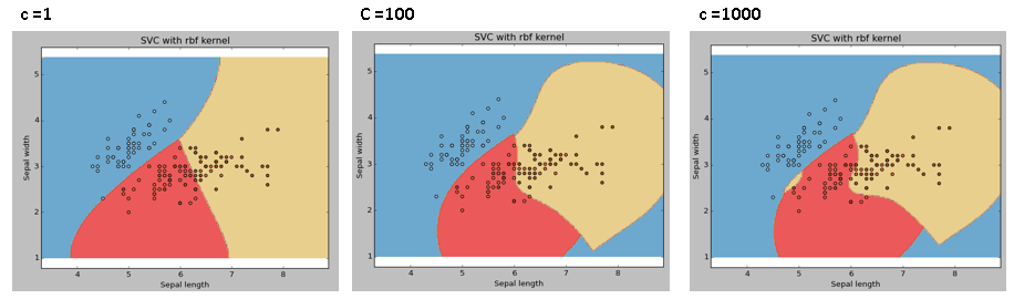
We should always look at the cross-validation score to effectively combine these parameters and avoid over-fitting.
In R, SVMs algorithm can be tuned in a similar fashion as they are in Python. Mentioned below are the respective parameters for the e1071 package:
Pros:
Cons:
Find the right additional feature to have a hyper-plane for segregating the classes in the below snapshot:
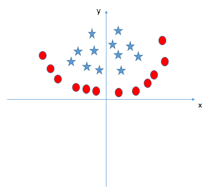
Answer the variable name in the comments section below. I’ll then reveal the answer.
In this article, we looked at the machine learning algorithm, Support Vector Machine, in detail. We discussed the concept of its working, the process of its implementation in python and R, and the tricks to make the model more efficient by tuning its parameters. Towards the end, we also pointed out the pros and cons of the algorithm. I suggest you try solving the problem above to practice your SVM algorithm skills and also try to analyze the power of this model by tuning the parameters.
Hope you found this information on Support Vector Machines, SVM classifiers, and their role in machine learning helpful and engaging!
Key Takeaways
A. Support vector machines (SVM) are supervised learning models used for classification and regression tasks. For instance, they can classify emails as spam or not spam. Additionally, they can be used to identify handwritten digits in image recognition.
A. The principle of SVM involves finding the hyperplane that best separates different classes of data. Essentially, it maximizes the margin between the closest points of the classes, thereby ensuring robust classification.
A. The function of SVM is to classify data by finding the optimal hyperplane that separates different classes. Consequently, it works well for both linear and non-linear classification problems by transforming data using kernel functions.
A. It is called a support vector machine because it relies on support vectors, which are the data points closest to the hyperplane. These support vectors are critical as they define the position and orientation of the hyperplane, thus influencing the model’s accuracy.
Sunil Ray is Chief Content Officer at Analytics Vidhya, India's largest Analytics community. I am deeply passionate about understanding and explaining concepts from first principles. In my current role, I am responsible for creating top notch content for Analytics Vidhya including its courses, conferences, blogs and Competitions. I thrive in fast paced environment and love building and scaling products which unleash huge value for customers using data and technology. Over the last 6 years, I have built the content team and created multiple data products at Analytics Vidhya. Prior to Analytics Vidhya, I have 7+ years of experience working with several insurance companies like Max Life, Max Bupa, Birla Sun Life & Aviva Life Insurance in different data roles. Industry exposure: Insurance, and EdTech Major capabilities: Content Development, Product Management, Analytics, Growth Strategy.
Lorem ipsum dolor sit amet, consectetur adipiscing elit,


hi, gr8 articles..explaining the nuances of SVM...hope u can reproduce the same with R.....it would be gr8 help to all R junkies like me
NEW VARIABLE (Z) = SQRT(X) + SQRT (Y)
Given problem Data points looks like y=x^2+c. So i guess z=x^2-y OR z=y-x^2.
i think x coodinates must increase after sqrt
Kernel
I mean kernel will add the new feature automatically.
Nicely Explained . The hyperplane to separate the classes for the above problem can be imagined as 3-D Parabola. z=ax^2 + by^2 + c
Thanks a lot for this great hands-on article!
Really impressive content. Simple and effective. It could be more efficient if you can describe each of the parameters and practical application where you faced non-trivial problem examples.
kernel
How does the python code look like if we are using LSSVM instead of SVM?
Polynomial kernel function?! for exzmple : Z= A(x^2) + B(y^2) + Cx + Dy + E
Hi Sunil. Great Article. However, there's an issue in the code you've provided. When i compiled the code, i got the following error: Name error: name 'h' is not defined. I've faced this error at line 16, which is: "xx, yy = np.meshgrid(np.arange(x_min, x_min, h), ...). Could you look into it and let me know how to fix it?
great explanation :) I think new variable Z should be x^2 + y.
Nice Articlel
The solution is analogue to scenario-5 if you replace y by y-k
Your SVM explanation and kernel definition is very simple, and easy to understand. Kudos for that effort.
Most intuitive explanation of multidimensional svm I have seen. Thank you!
what is 'h' in the code of SVM . xx, yy = np.meshgrid(np.arange(x_min, x_max, h), np.arange(y_min, y_max, h))
z = (x^2 - y) z > 0, red circles
very neat explaination to SVC. For the proposed problem, my answers are: (1) z = a* x^2 + b y + c, a parabola. (2) z = a (x-0)^2 + b (y- y0)^2 - R^2, a circle or an ellipse enclosing red stars.
Great article.. I think the below formula would give a new variable that help to separate the points in hyper plane z = y - |x|
THANKS FOR EASY EXPLANATION
Useful article for Machine learners.. Why can't you discuss about effect of kernel functions.
The explanation is really impressive. Can you also provide some information about how to determine the theoretical limits for the parameter's optimal accuracy.
how can we use SVM for regression? can someone please explain..
hi please if you have an idiea about how it work for regression can you help me ?
That was a really good explanation! thanks a lot. I read many explanations about SVM but this one help me to understand the basics which I really needed it.
please give us the answer
This is very useful for understanding easily.
just substitude x with |x|
Same goes with Diana. This really help me a lot to figure out things from basic. I hope you would also share any computation example using R provided with simple dataset, so that anyone can practice with their own after referring to your article. I have a question, if i have time-series dataset containing mixed linear and nonlinear data, (for example oxygen saturation data ; SaO2), by using svm to do classification for diseased vs health subjects, do i have to separate those data into linear and non-linear fisrt, or can svm just performed the analysis without considering the differences between the linearity of those data? Thanks a lot!
z
Could you please explain how SVM works for multiple classes? How would it work for 9 classes? I used a function called multisvm here: http://www.mathworks.com/matlabcentral/fileexchange/39352-multi-class-svm but I'm not sure how it's working behind the scenes. Everything I've read online is rather confusing.
NEW VARIABLE (Z) = SQRT(X) + SQRT (Y)
Thank you so much!! That is really good explanation! I read many explanations about SVM but this one help me to understand the basics which I really needed it. keep it up!!
Thanks for the great article. There are even cool shirts for anyone who became SVM fan ;) http://www.redbubble.com/de/people/perceptron/works/24728522-support-vector-machines?grid_pos=2&p=t-shirt&style=mens
great explanation!! Thanks for posting it.
I think this is |X|
It is very nicely written and understandable. Thanks a lot...
z=ax^2 + by^2
nice explanations with scenarios and margin values
wow!!! excellent explanation.. only now i understood the concepts clearly thanks a lot..
(Z) = SQRT(X) + SQRT (Y)
thanks, and well done for the good article
it's magnific your explanation
Great Explanation..Thanks..
simple and refreshed the core concepts in just 5 mins! kudos Mr.Sunil
Best starters material for SVM, really appreciate the simple and comprehensive writing style. Expecting more such articles from you
Z= square(x)
Hey Sunil, Nice job of explaining it concisely and intuitively! Easy to follow and covers many aspects in a short space. Thanks!
Very well written - concise, clear, well-organized. Thank you.
Bonjour, je souhaite appliquer cet algorithme à mes données puis afficher le résultat. Je ne maîtrise pas très bien python, j'ai donc recopié le code suivant: def pro_svc(X): # we create an instance of SVM and fit out data. We do not scale our # data since we want to plot the support vectors C = 1.0 # SVM regularization parameter svc = svm.SVC(kernel='linear', C=1,gamma=0).fit(X, y) # create a mesh to plot in x_min, x_max = X[:, 0].min() - 1, X[:, 0].max() + 1 y_min, y_max = X[:, 1].min() - 1, X[:, 1].max() + 1 h = (x_max / x_min)/100 xx, yy = np.meshgrid(np.arange(x_min, x_max, h), np.arange(y_min, y_max, h)) #repartition d'un nobre de points entre un start et un end plt.subplot(1, 1, 1) Z = svc.predict(np.c_[xx.ravel(), yy.ravel()]) Z = Z.reshape(xx.shape) plt.contourf(xx, yy, Z, cmap=plt.cm.Paired, alpha=0.8) plt.scatter(X[:, 0], X[:, 1], c=y, cmap=plt.cm.Paired) plt.xlabel('Sepal length') plt.ylabel('Sepal width') plt.xlim(xx.min(), xx.max()) plt.title('SVC with linear kernel') plt.show() Lorque j'appelle ce code sur me données (matrices numpy 60 lignes, 2 colonnes) l'erreur suivante s'affiche : ValueError: zero-size array to reduction operation maximum which has no identity Que dois_je faire ? Merci d'avance pour votre aide
Oh sorry should have asked my question in english... The code I sent in my first comment is the code I took from this website and I cannot manage to make it work, I always got this message when I call the function "ValueError: zero-size array to reduction operation maximum which has no identity" What should I do? Thank you in advance
Excellent explanation..Can you please also tell what are the parameter values one should start with - like C, gamma ..Also, again a very basic question.. Can we say that lesser the % of support vectors (count of SVs/total records) better my model/richer my data is- assuming the datasize to be the same.. Waiting for more on parameter tuning..Really appreciate the knowledge shared..
Hi could you please explain why SVM perform well on small dataset?
Another nice kernel for the problem stated in the article is the radial basis kernel.
[…] 资源:阅读这篇文章来理解SVM support vector machines。 […]
wow excellent
very appreciating for explaining
Nice tutorial. The new feature to separate data would be something like z = y - x^2 as most dots following the parabola will have lower z than stars.
Very intuitive explanation. Thank you! Good to add SVM for Regression of Continuous variables.
this is so simple method that anyone can get easily thnx for that but also explain the 4 senario of svm.
Great article for understanding of SVM: But, When and Why do we use the SVM algorithm can anyone make that help me understand because until this thing is clear there may not be use of this article. Thanks in advance.
It is one of best explanation of machine learning technique that i have seen! and new variable: i think Z=|x| and new Axis are Z and Y
higher degree polynomial will separate the points in the problem,
I guess the required feature is z = x^2 / y^2 For the red points, z will be close to 1 but for the blue points z values will be significantly more than 1
amazing article no doubt! It makes me clear all the concept and deep points regarding SVM. many thanks.
The best explanation ever! Thank you!
z = x^2+y^2
[…] [1] Naive Bayes and Text Classification. [2]Naive Bayes by Example. [3] Andrew Ng explanation of Naive Bayes video 1 and video 2 [4] Please explain SVM like I am 5 years old. [5] Understanding Support Vector Machines from examples. […]
new variable = ABS(Y)
Man, I was looking for definition of SVM for my diploma, but I got interested in explanation part of this article. Keep up good work!
we can use 'poly' kernel with degree=2
Hi.. Very well written, great article !:). Thanks so much share knowledge on SVM.
z=y-x^2
Wonderful, easy to understand explanation.
Thanks a lot for your explanations, they were really helpful and easy to understand
Really helpful article. Can you please elaborate on time complexity for implementation of SVMs? Are they polynomial time or non-polynomial time executing algorithms?
Good explanation,but it would be better if some one explains the equations and math formulation involved in SVM. y=w.x+b
It would be a parabola z = a*x^2 + b*y^2 + c*x + d*y + e
Very good explanation, helpful
valuable explanation!!
Thanks for your great overview and explanation about SVM's!! Only one question: In the very beginning you define what a Support Vector is. Shouldn't you emphasize, that it is only a subset of the data points? Otherwise you could wonder if all data points are Support Vectors. Cheers, Lena
Very helpfull
ValueError: The gamma value of 0.0 is invalid. Use 'auto' to set gamma to a value of 1 / n_features.
Thanks for the great article. I have a question...for data like tweets of twitter....svm is helpful or it would be better to choose another option? which will be helpful?.
I would do |x| or 2 linear SVMs -ax+b, till 0 and then cx+d afterward. Concatenating linear SVM is way more powerful than expected. A very nice explanation, I totally love your work.
I think you should change the title "How to implement SVM in Python and R?" because you don't actually implement SVM, you only use implementations of SVM through some libraries like scikit-learn for Python.
|X|
thank u sir ,it is easy to understand
Hi Sunil, Great explanation of SVM in very simple and understandable format. Can you please the equivalent R code for generating the mesh plots? I think the hyper-plane looks like a parabola. So the new feature is z = y^2+y+x^2+x+c. Kindly let me know if this is correct. Thanks & Regards, Pallavi
Hi Sunil, Wonderful article. Can you also cover what are gamma and cost values and how to select them?
z = x^2 + y
Hi there. Great article. I have a question. You wrote: "if you have large number of features (>1000) because it is more likely that the data is linearly separable in high dimensional space." Could you explain why this is probably the case? Thanks
Hello, great article there. Just one quesiton. You wrote: "if you have large number of features (>1000) because it is more likely that the data is linearly separable in high dimensional space" Could you explain why this is probably the case? Thanks
It may be z=x^2+y
y=x^2
z=ax^2 + by^2 + c
Nice. new variable is z = abs(x). Then replace x coordinates with z coordinates
Can you please tell me how an image can be represented as a single point in support vector space..... and how histograms used in support vector classification... I know it is not related to this article... but I am asking in general...
z = |x|
My God, your English is so broken!
PARABOLA
I think the boundaryf between two type of snapshot could be a curve (of a part of circle). So I prefer kernel Z=sqrt(X^2+(Y-c)^2)
Thanks a lot. I like how you define a problem and then solve it. It makes things clear.
hi, can anyone help me for forecasting of stock exchange by SVM in rstudio, i hv a project for my mphil course work.
z=x-y^2
The content is good but you can not use the gamma parameter if you want to separate your data linearly.
explanations are easy to undersdand
Polynomial kernel, Nice and simple explanation with required knowledge
Really good article.
This is great article. And the explanation are clear
New Variable (z) = x**2 - y + c (some constant)
z = x**2 - y + c (some constant)