Introduction
A a Python library emerges with the capacity to revolutionize the deep learning landscape, and PyTorch Tutorial and PyTorch Guide are prime examples of this phenomenon. Over the past few weeks, I’ve delved into PyTorch, and I’ve been astounded by its intuitive nature. Among the array of deep learning frameworks I’ve encountered, PyTorch stands out as the most flexible and effortless to grasp.
Note – This article assumes that you have a basic understanding of deep learning. If you want to get up to speed with deep learning, please go through this article first.
Also, if you want a more detailed explanation of PyTorch from scratch, understand how tensors works, how you can perform mathematical as well as matrix operations using PyTorch, I highly recommend checking out A Beginner-Friendly Guide to PyTorch and How it Works from Scratch
If you prefer to approach the following concepts in a structured format, you can enrol for this free course on PyTorch and follow them chapter-wise.
Table of contents
An Overview of PyTorch
PyTorch’s creators say that they have a philosophy – they want to be imperative. This means that we run our computation immediately. This fits right into the python programming methodology, as we don’t have to wait for the whole code to be written before getting to know if it works or not. We can easily run a part of the code and inspect it in real time. For me as a neural network debugger, this is a blessing!
PyTorch is a python based library built to provide flexibility as a deep learning development platform. The workflow of PyTorch is as close as you can get to python’s scientific computing library – numpy.
Now you might ask,
Why Would we Use PyTorch Guide to Build Deep Learning Models
- Easy to use API – It is as simple as python can be.
- Python support – As mentioned above, PyTorch smoothly integrates with the python data science stack. It is so similar to numpy that you might not even notice the difference.
- Dynamic computation graphs – Instead of predefined graphs with specific functionalities, PyTorch provides a framework for us to build computational graphs as we go, and even change them during runtime. This is valuable for situations where we don’t know how much memory is going to be required for creating a neural network.
A few other advantages of using PyTorch are it’s multiGPU support, custom data loaders and simplified preprocessors.
Since its release in the start of January 2016, many researchers have adopted it as a go-to library because of its ease of building novel and even extremely complex graphs. Having said that, there is still some time before PyTorch is adopted by the majority of data science practitioners due to it’s new and “under construction” status.
Diving into the Technicalities
Before diving into the details, let us go through the workflow of PyTorch.
PyTorch uses an imperative / eager paradigm. That is, each line of code required to build a graph defines a component of that graph. We can independently perform computations on these components itself, even before your graph is built completely. This is called “define-by-run” methodology.
Installing PyTorch is pretty easy. You can follow the steps mentioned in the official docs and run the command as per your system specifications. For example, this was the command I used on the basis of the options I chose:
conda install pytorch torchvision cuda91 -c pytorchThe main elements we should get to know when starting out with PyTorch are:
- PyTorch Tensors
- Mathematical Operations
- Autograd module
- Optim module and
- nn module
Below, we’ll take a look at each one in some detail.
PyTorch Tensors
Tensors are nothing but multidimensional arrays. Tensors in PyTorch are similar to numpy’s ndarrays, with the addition being that Tensors can also be used on a GPU. PyTorch supports various types of Tensors. If you are familiar with other deep learning frameworks, you must have come across tensors in TensorFlow as well. In fact, you are welcome to implement the following tasks in Tensorflow too and make your own comparison of PyTorch vs. TensorFlow!
You can define a simple one dimensional matrix as below:
# import pytorch
import torch

# define a tensor
torch.FloatTensor([2])
2
[torch.FloatTensor of size 1]Mathematical Operations
As with numpy, it is very crucial that a scientific computing library has efficient implementations of mathematical functions. Pytorch Guide gives you a similar interface, with more than 200+ mathematical operations you can use.
Below is an example of a simple addition operation in PyTorch:
a = torch.FloatTensor([2])
b = torch.FloatTensor([3])

a + b
5
[torch.FloatTensor of size 1]Doesn’t this look like a quinessential python approach? We can also perform various matrix operations on the PyTorch tensors we define. For example, we’ll transpose a two dimensional matrix:
matrix = torch.randn(3, 3)
matrix

0.7162 1.0152 1.1525
-0.3503 -0.9452 -1.0861
-0.1093 -0.0927 -0.0476
matrix.t()
0.7162 -0.3503 -0.1093
1.0152 -0.9452 -0.0927
1.1525 -1.0861 -0.0476
[torch.FloatTensor of size 3x3]Autograd module
Pytorch Guide uses a technique called automatic differentiation. That is, we have a recorder that records what operations we have performed, and then it replays it backward to compute our gradients. This technique is especially powerful when building neural networks, as we save time on one epoch by calculating differentiation of the parameters at the forward pass itself.
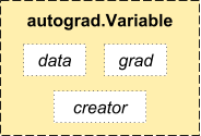
from torch.autograd import Variable

x = Variable(train_x)
y = Variable(train_y, requires_grad=False)
Optim module
torch.optim is a module that implements various optimization algorithms used for building neural networks. Most of the commonly used methods are already supported, so that we don’t have to build them from scratch (unless you want to!).
Below is the code for using an Adam optimizer:
optimizer = torch.optim.Adam(model.parameters(), lr=learning_rate)nn module
Pytorch Guide autograd makes it easy to define computational graphs and take gradients, but raw autograd can be a bit too low-level for defining complex neural networks. This is where the nn module can help.
The nn package defines a set of modules, which we can think of as a neural network layer that produces output from input and may have some trainable weights.
You can consider a nn module as the keras of PyTorch!
import torch

# define model
model = torch.nn.Sequential(
 torch.nn.Linear(input_num_units, hidden_num_units),
 torch.nn.ReLU(),
 torch.nn.Linear(hidden_num_units, output_num_units),
)
loss_fn = torch.nn.CrossEntropyLoss()
Now that you know the basic components of PyTorch, you can easily build your own neural network from scratch. Follow along if you want to know how!
Building a neural network in Numpy vs. PyTorch
I have mentioned previously that PyTorch and Numpy are remarkably similar. Let’s look at why. In this section, we’ll see an implementation of a simple neural network to solve a binary classification problem (you can go through this article for it’s in-depth explanation).
## Neural network in numpy

import numpy as np

#Input array
X=np.array([[1,0,1,0],[1,0,1,1],[0,1,0,1]])

#Output
y=np.array([[1],[1],[0]])

#Sigmoid Function
def sigmoid (x):
 return 1/(1 + np.exp(-x))

#Derivative of Sigmoid Function
def derivatives_sigmoid(x):
 return x * (1 - x)

#Variable initialization
epoch=5000 #Setting training iterations
lr=0.1 #Setting learning rate
inputlayer_neurons = X.shape[1] #number of features in data set
hiddenlayer_neurons = 3 #number of hidden layers neurons
output_neurons = 1 #number of neurons at output layer

#weight and bias initialization
wh=np.random.uniform(size=(inputlayer_neurons,hiddenlayer_neurons))
bh=np.random.uniform(size=(1,hiddenlayer_neurons))
wout=np.random.uniform(size=(hiddenlayer_neurons,output_neurons))
bout=np.random.uniform(size=(1,output_neurons))

for i in range(epoch):
  #Forward Propogation
  hidden_layer_input1=np.dot(X,wh)
  hidden_layer_input=hidden_layer_input1 + bh
  hiddenlayer_activations = sigmoid(hidden_layer_input)
  output_layer_input1=np.dot(hiddenlayer_activations,wout)
  output_layer_input= output_layer_input1+ bout
  output = sigmoid(output_layer_input)

  #Backpropagation
  E = y-output
  slope_output_layer = derivatives_sigmoid(output)
  slope_hidden_layer = derivatives_sigmoid(hiddenlayer_activations)
  d_output = E * slope_output_layer
  Error_at_hidden_layer = d_output.dot(wout.T)
  d_hiddenlayer = Error_at_hidden_layer * slope_hidden_layer
  wout += hiddenlayer_activations.T.dot(d_output) *lr
  bout += np.sum(d_output, axis=0,keepdims=True) *lr
  wh += X.T.dot(d_hiddenlayer) *lr
  bh += np.sum(d_hiddenlayer, axis=0,keepdims=True) *lr

print('actual :\n', y, '\n')
print('predicted :\n', output)
Now, try to spot the difference in a super simple implementation of the same in PyTorch (the differences are mentioned in bold in the below code).
## neural network in pytorch
import torch

#Input array
X = torch.Tensor([[1,0,1,0],[1,0,1,1],[0,1,0,1]])

#Output
y = torch.Tensor([[1],[1],[0]])

#Sigmoid Function
def sigmoid (x):
  return 1/(1 + torch.exp(-x))

#Derivative of Sigmoid Function
def derivatives_sigmoid(x):
  return x * (1 - x)

#Variable initialization
epoch=5000 #Setting training iterations
lr=0.1 #Setting learning rate
inputlayer_neurons = X.shape[1] #number of features in data set
hiddenlayer_neurons = 3 #number of hidden layers neurons
output_neurons = 1 #number of neurons at output layer

#weight and bias initialization
wh=torch.randn(inputlayer_neurons, hiddenlayer_neurons).type(torch.FloatTensor)
bh=torch.randn(1, hiddenlayer_neurons).type(torch.FloatTensor)
wout=torch.randn(hiddenlayer_neurons, output_neurons)
bout=torch.randn(1, output_neurons)

for i in range(epoch):

  #Forward Propogation
  hidden_layer_input1 = torch.mm(X, wh)
  hidden_layer_input = hidden_layer_input1 + bh
  hidden_layer_activations = sigmoid(hidden_layer_input)

  output_layer_input1 = torch.mm(hidden_layer_activations, wout)
  output_layer_input = output_layer_input1 + bout
  output = sigmoid(output_layer_input1)

  #Backpropagation
  E = y-output
  slope_output_layer = derivatives_sigmoid(output)
  slope_hidden_layer = derivatives_sigmoid(hidden_layer_activations)
  d_output = E * slope_output_layer
  Error_at_hidden_layer = torch.mm(d_output, wout.t())
  d_hiddenlayer = Error_at_hidden_layer * slope_hidden_layer
  wout += torch.mm(hidden_layer_activations.t(), d_output) *lr
  bout += d_output.sum() *lr
  wh += torch.mm(X.t(), d_hiddenlayer) *lr
  bh += d_output.sum() *lr

print('actual :\n', y, '\n')
print('predicted :\n', output)
Comparison with other deep learning libraries
In one benchmarking script, it is successfully shown that PyTorch outperforms all other major deep learning libraries in training a Long Short Term Memory (LSTM) network by having the lowest median time per epoch (refer to the image below).
The APIs for data loading are well designed in PyTorch. The interfaces are specified in a dataset, a sampler, and a data loader.
On comparing the tools for data loading in TensorFlow (readers, queues, etc.), I found PyTorch‘s data loading modules pretty easy to use. Also, PyTorch is seamless when we try to build a neural network, so we don’t have to rely on third party high-level libraries like keras.
On the other hand, I would not yet recommend using PyTorch for deployment. PyTorch is yet to evolve. As the PyTorch developers have said, “What we are seeing is that users first create a PyTorch model. When they are ready to deploy their model into production, they just convert it into a Caffe 2 model, then ship it into either mobile or another platform.”
Case Study – Solving an Image Recognition problem in PyTorch
To get familiar with PyTorch, we will solve Analytics Vidhya’s deep learning practice problem – Identify the Digits. Let’s take a look at our problem statement:
Our problem is an image recognition problem, to identify digits from a given 28 x 28 image. We have a subset of images for training and the rest for testing our model.
So first, download the train and test files. The dataset contains a zipped file of all the images and both the train.csv and test.csv have the name of corresponding train and test images. Any additional features are not provided in the datasets, just the raw images are provided in ‘.png’ format.
Let’s begin:
STEP 0: Getting Ready
a) Import all the necessary libraries
# import modules
%pylab inline
import os
import numpy as np
import pandas as pd
from scipy.misc import imread
from sklearn.metrics import accuracy_score
b) Let’s set a seed value, so that we can control our models randomness
# To stop potential randomness
seed = 128
rng = np.random.RandomState(seed)
c) The first step is to set directory paths, for safekeeping!
root_dir = os.path.abspath('.')
data_dir = os.path.join(root_dir, 'data')

# check for existence
os.path.exists(root_dir), os.path.exists(data_dir)
STEP 1: Data Loading and Preprocessing
a) Now let us read our datasets. These are in .csv formats, and have a filename along with the appropriate labels
# load dataset
train = pd.read_csv(os.path.join(data_dir, 'Train', 'train.csv'))
test = pd.read_csv(os.path.join(data_dir, 'Test.csv'))

sample_submission = pd.read_csv(os.path.join(data_dir, 'Sample_Submission.csv'))

train.head()| filename | label | |
|---|---|---|
| 0 | 0.png | 4 |
| 1 | 1.png | 9 |
| 2 | 2.png | 1 |
| 3 | 3.png | 7 |
| 4 | 4.png | 3 |
b) Let us see what our data looks like! We read our image and display it.
# print an image
img_name = rng.choice(train.filename)
filepath = os.path.join(data_dir, 'Train', 'Images', 'train', img_name)

img = imread(filepath, flatten=True)

pylab.imshow(img, cmap='gray')
pylab.axis('off')
pylab.show()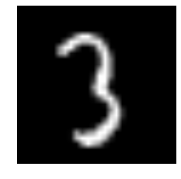
d) For easier data manipulation, let’s store all our images as numpy arrays
# load images to create train and test set
temp = []
for img_name in train.filename:
  image_path = os.path.join(data_dir, 'Train', 'Images', 'train', img_name)
  img = imread(image_path, flatten=True)
  img = img.astype('float32')
  temp.append(img)

train_x = np.stack(temp)

train_x /= 255.0
train_x = train_x.reshape(-1, 784).astype('float32')

temp = []
for img_name in test.filename:
  image_path = os.path.join(data_dir, 'Train', 'Images', 'test', img_name)
  img = imread(image_path, flatten=True)
  img = img.astype('float32')
  temp.append(img)

test_x = np.stack(temp)

test_x /= 255.0
test_x = test_x.reshape(-1, 784).astype('float32')

train_y = train.label.values
e) As this is a typical ML problem, to test the proper functioning of our model we create a validation set. Let’s take a split size of 70:30 for train set vs validation set
# create validation set
split_size = int(train_x.shape[0]*0.7)

train_x, val_x = train_x[:split_size], train_x[split_size:]
train_y, val_y = train_y[:split_size], train_y[split_size:]
STEP 2: Model Building
a) Now comes the main part! Let us define our neural network architecture. We define a neural network with 3 layers input, hidden and output. The number of neurons in input and output are fixed, as the input is our 28 x 28 image and the output is a 10 x 1 vector representing the class. We take 50 neurons in the hidden layer. Here, we use Adam as our optimization algorithms, which is an efficient variant of Gradient Descent algorithm.
import torch
from torch.autograd impoxrt Variable
# number of neurons in each layer
input_num_units = 28*28
hidden_num_units = 500
output_num_units = 10
# set remaining variables
epochs = 5
batch_size = 128
learning_rate = 0.001b) It’s time to train our model
# define model
model = torch.nn.Sequential(
  torch.nn.Linear(input_num_units, hidden_num_units),
  torch.nn.ReLU(),
  torch.nn.Linear(hidden_num_units, output_num_units),
)
loss_fn = torch.nn.CrossEntropyLoss()

# define optimization algorithm
optimizer = torch.optim.Adam(model.parameters(), lr=learning_rate)
## helper functions
# preprocess a batch of dataset
def preproc(unclean_batch_x):
"""Convert values to range 0-1"""
temp_batch = unclean_batch_x / unclean_batch_x.max()
return temp_batch
# create a batch
def batch_creator(batch_size):
dataset_name = 'train'
dataset_length = train_x.shape[0]
batch_mask = rng.choice(dataset_length, batch_size)
batch_x = eval(dataset_name + '_x')[batch_mask]
batch_x = preproc(batch_x)
if dataset_name == 'train':
batch_y = eval(dataset_name).ix[batch_mask, 'label'].values
return batch_x, batch_y# train network
total_batch = int(train.shape[0]/batch_size)
for epoch in range(epochs):
avg_cost = 0
for i in range(total_batch):
# create batch
batch_x, batch_y = batch_creator(batch_size)
# pass that batch for training
x, y = Variable(torch.from_numpy(batch_x)), Variable(torch.from_numpy(batch_y), requires_grad=False)
pred = model(x)
# get loss
loss = loss_fn(pred, y)
# perform backpropagation
loss.backward()
optimizer.step()
avg_cost += loss.data[0]/total_batch
print(epoch, avg_cost)# get training accuracy
x, y = Variable(torch.from_numpy(preproc(train_x))), Variable(torch.from_numpy(train_y), requires_grad=False)
pred = model(x)
final_pred = np.argmax(pred.data.numpy(), axis=1)
accuracy_score(train_y, final_pred)# get validation accuracy
x, y = Variable(torch.from_numpy(preproc(val_x))), Variable(torch.from_numpy(val_y), requires_grad=False)
pred = model(x)
final_pred = np.argmax(pred.data.numpy(), axis=1)
accuracy_score(val_y, final_pred)
The training score comes out to be:0.8779008746355685
whereas, the validation score is:0.867482993197279
This is a pretty impressive score especially when we have trained a very simple neural network for just five epochs!
Conclusion
PyTorch simplifies deep learning model development with its intuitive and Pythonic APIs. Its dynamic computation graphs, seamless integration with Python data science stack, and efficient GPU support make it a powerful choice. Although relatively new, PyTorch has gained traction among researchers for building innovative neural network architectures. With its user-friendly ecosystem, comprehensive documentation, and active community support, Pytorch Guide empowers both beginners and experts to prototype, experiment, and deploy deep learning solutions efficiently. As the library continues evolving, PyTorch holds immense potential to drive further advancements in the field of machine learning and artificial intelligence.
Frequently Asked Questions?
Q1. Is PyTorch easy to learn?
A. PyTorch is considered relatively easy to learn, especially for those already familiar with Python and deep learning concepts. Its dynamic computation graph and intuitive syntax make it accessible for beginners. However, like any new framework or library, it requires practice and dedication to fully grasp its capabilities and effectively apply them.
Q2. What PyTorch is used for?
A. PyTorch is primarily used for building deep learning models and conducting research in the field of artificial intelligence. It provides a flexible and efficient platform for developing neural networks, including convolutional neural networks (CNNs), recurrent neural networks (RNNs), and transformer models. Pytorch Guide is also widely used for tasks such as image classification, natural language processing, reinforcement learning, and computer vision.
Q3. Is PyTorch written in C or C++?
A. PyTorch is primarily implemented in C++ for efficiency and performance. However, it offers Python bindings that allow developers to interact with the underlying C++ code using Python syntax. This combination of C++ core functionality and Python interface makes PyTorch both powerful and accessible.
Q4. Can I learn PyTorch from scratch?
A. Yes, you can learn Pytorch Guide from scratch, especially if you have a basic understanding of Python programming and fundamental concepts of deep learning. There are numerous resources available, including official documentation, tutorials, online courses, and community forums, that can help you get started with PyTorch. Starting with simple examples and gradually building up your knowledge through experimentation and practice is an effective way to learn PyTorch from scratch.
JalFaizy Shaikh
22 Mar, 2024
Faizan is a Data Science enthusiast and a Deep learning rookie. A recent Comp. Sc. undergrad, he aims to utilize his skills to push the boundaries of AI research.


I believe your derivative of sigmoid function should actually be: def derivatives_sigmoid(x): return sigmoid(x)*(1-sigmoid(x)) As per: https://beckernick.github.io/sigmoid-derivative-neural-network/
Thanks a lot for your nice and compact introduction on pytorch. Just a little mistake I spotted: In the Mathematical Operations section, you do not use the same matrix to show how the transpose operation works, i.e. matrix.t() is not the transpose of the matrix you earlier defined.
Thanks for pointing it out. I have updated the article
Nice article Faizan. I am confused regarding the concept of an epoch. Doesn't one epoch mean we have gone through all the training examples once? But it seems that you are doing a batch selection with replacement. batch_mask = rng.choice(dataset_length, batch_size) Would this make sure that all training examples are seen in one epoch?
Faizen is using minibatches here. In theory, yes, an epoch is supposed to take one step in the average direction of the negative gradient of the entire training set. But that's expensive and slow, and it's a good trade to use minibatches with only a subset of the training set. Choosing with replacement is a bit odd though - I would have shuffled the training set and then iterated through it in chunks.
I cannot understand how pytorch could calculate differentiation of the parameters at the forward pass itself. Can you please share the source of this information mentioned in your article? Thanks.
Hey - you can take a look at how PyTorch's autograd package works internally (http://pytorch.org/docs/master/notes/autograd.html)
Very nice tutorial !!!!! Just one input, please provide dataset link as well you used in this example.
Hi , Can you kindly explain whya are we doing wout = wout + lr* gradient ? we are minimising the function so shouldn't we do wout = wout - learning_rate*gradient ?