Introduction
Ensemble techniques in machine learning function much like seeking advice from multiple sources before making a significant decision, such as purchasing a car. Just as you wouldn’t rely solely on one opinion, ensemble models combine predictions from multiple base models to enhance overall performance. One popular method, majority voting, aggregates predictions to select the class label by majority. This tutorial explores ensemble learning concepts, including bootstrap sampling to train models on different subsets, the role of predictors in building diverse models, and practical implementation in Python using scikit-learn.
It addresses binary classification scenarios and delves into techniques to tackle issues like data mining, which identifies valuable patterns from data, and managing high variance through ensemble methods. Additionally, the tutorial covers optimizing ensemble performance with hyperparameter tuning, providing a comprehensive foundation for leveraging ensemble learning effectively.
Are you a beginner looking for a place to start your journey in data science and machine learning? Presenting two comprehensive courses, full of knowledge and data science learning, curated just for you!
Learning Outcomes
- Understand the principles and algorithms behind various machine learning models and neural networks.
- Implement machine learning models and neural networks to solve real-world problems.
- Analyze and interpret the predictive performance of machine learning models and neural networks.
- Explain the concept of stacked generalization and its use in improving model accuracy.
- Perform exploratory data analysis and data preprocessing to prepare datasets for modeling.
- Apply feature selection methods to reduce dimensionality and improve model efficiency.
- Compare and contrast different learning methods, such as supervised, unsupervised, and reinforcement learning.
- Implement popular ensemble techniques, including bagging, boosting, and stacking, to improve model performance.
This article was published as a part of the Data Science Blogathon.
Table of contents
What is Ensemble Learning with example?
Ensemble learning is a machine learning technique that enhances accuracy and resilience in forecasting by merging predictions from multiple models. It aims to mitigate errors or biases that may exist in individual models by leveraging the collective intelligence of the ensemble.
The underlying concept behind ensemble learning is to combine the outputs of diverse models to create a more precise prediction. By considering multiple perspectives and utilizing the strengths of different models, ensemble learning improves the overall performance of the learning system. This approach not only enhances accuracy but also provides resilience against uncertainties in the data. By effectively merging predictions from multiple models, ensemble learning has proven to be a powerful tool in various domains, offering more robust and reliable forecasts.
Let’s understand the concept of ensemble learning with an example. Suppose you are a movie director and you have created a short movie on a very important and interesting topic. Now, you want to take preliminary feedback (ratings) on the movie before making it public.
Possible Ways
A: You may ask one of your friends to rate the movie for you.
Now it’s entirely possible that the person you have chosen loves you very much and doesn’t want to break your heart by providing a 1-star rating to the horrible work you have created.
B: Another way could be by asking 5 colleagues of yours to rate the movie.
This should provide a better idea of the movie. This method may provide honest ratings for your movie. But a problem still exists. These 5 people may not be “Subject Matter Experts” on the topic of your movie. Sure, they might understand the cinematography, the shots, or the audio, but at the same time may not be the best judges of dark humor.
C: How about asking 50 people to rate the movie?
Some of which can be your friends, some of them can be your colleagues and some may even be total strangers.
The responses, in this case, would be more generalized and diversified since now you have people with different sets of skills. And as it turns out – this is a better approach to get honest ratings than the previous cases we saw.
With these examples, you can infer that a diverse group of people are likely to make better decisions as compared to individuals. Similar is true for a diverse set of models in comparison to single models. This diversification in Machine Learning is achieved by a technique called Ensemble Learning.
Now that you have got a gist of what ensemble learning is – let us look at the various techniques in ensemble learning along with their implementations.
Simple Ensemble Techniques
In this section, we will look at a few simple but powerful techniques, namely:
- Max Voting
- Averaging
- Weighted Averaging
Max Voting
The max voting method is generally used for classification problems. In this technique, multiple models are used to make predictions for each data point. The predictions by each model are considered as a ‘vote’. The predictions which we get from the majority of the models are used as the final prediction.
For example, when you asked 5 of your colleagues to rate your movie (out of 5); we’ll assume three of them rated it as 4 while two of them gave it a 5. Since the majority gave a rating of 4, the final rating will be taken as 4. You can consider this as taking the mode of all the predictions.
The result of max voting would be something like this:
| Colleague 1 | Colleague 2 | Colleague 3 | Colleague 4 | Colleague 5 | Final rating |
| 5 | 4 | 5 | 4 | 4 | 4 |
Sample Code:
Here x_train consists of independent variables in training data, y_train is the target variable for training data. The validation set is x_test (independent variables) and y_test (target variable) .
Alternatively, you can use “VotingClassifier” module in sklearn as follows:
from sklearn.ensemble import VotingClassifier
model1 = LogisticRegression(random_state=1)
model2 = tree.DecisionTreeClassifier(random_state=1)
model = VotingClassifier(estimators=[('lr', model1), ('dt', model2)], voting='hard')
model.fit(x_train,y_train)
model.score(x_test,y_test)
Averaging
Similar to the max voting technique, multiple predictions are made for each data point in averaging. In this method, we take an average of predictions from all the models and use it to make the final prediction. Averaging can be used for making predictions in regression problems or while calculating probabilities for classification problems.
For example, in the below case, the averaging method would take the average of all the values.
i.e. (5+4+5+4+4)/5 = 4.4
| Colleague 1 | Colleague 2 | Colleague 3 | Colleague 4 | Colleague 5 | Final rating |
| 5 | 4 | 5 | 4 | 4 | 4.4 |
Sample Code:
model1 = tree.DecisionTreeClassifier()
model2 = KNeighborsClassifier()
model3= LogisticRegression()

model1.fit(x_train,y_train)
model2.fit(x_train,y_train)
model3.fit(x_train,y_train)

pred1=model1.predict_proba(x_test)
pred2=model2.predict_proba(x_test)
pred3=model3.predict_proba(x_test)

finalpred=(pred1+pred2+pred3)/3
Weighted Average
This is an extension of the averaging method. All models are assigned different weights defining the importance of each model for prediction. For instance, if two of your colleagues are critics, while others have no prior experience in this field, then the answers by these two friends are given more importance as compared to the other people.
The result is calculated as [(5*0.23) + (4*0.23) + (5*0.18) + (4*0.18) + (4*0.18)] = 4.41.
| Colleague 1 | Colleague 2 | Colleague 3 | Colleague 4 | Colleague 5 | Final rating | |
| weight | 0.23 | 0.23 | 0.18 | 0.18 | 0.18 | |
| rating | 5 | 4 | 5 | 4 | 4 | 4.41 |
Sample Code:
model1 = tree.DecisionTreeClassifier()
model2 = KNeighborsClassifier()
model3= LogisticRegression()

model1.fit(x_train,y_train)
model2.fit(x_train,y_train)
model3.fit(x_train,y_train)

pred1=model1.predict_proba(x_test)
pred2=model2.predict_proba(x_test)
pred3=model3.predict_proba(x_test)

finalpred=(pred1*0.3+pred2*0.3+pred3*0.4)
Advanced Ensemble techniques
Now that we have covered the basic ensemble techniques, let’s move on to understanding the advanced techniques.
Stacking
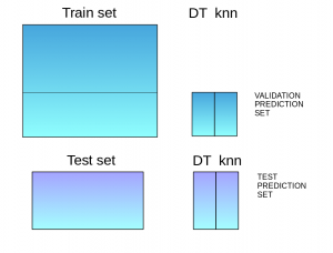
Stacking is an ensemble learning technique that uses predictions from multiple models (for example decision tree, knn or svm) to build a new model. This model is used for making predictions on the test set. Below is a step-wise explanation for a simple stacked ensemble:
- The train set is split into 10 parts.
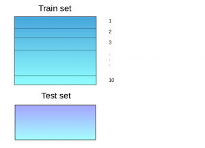
- A base model (suppose a decision tree) is fitted on 9 parts and predictions are made for the 10th part. This is done for each part of the train set.
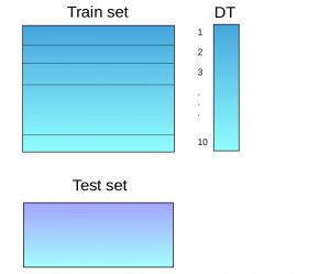
- The base model (in this case, decision tree) is then fitted on the whole train dataset.
- Using this model, predictions are made on the test set.
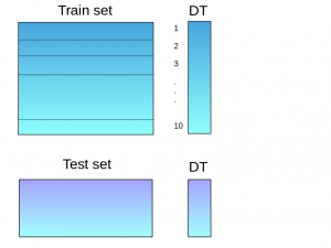
- Steps 2 to 4 are repeated for another base model (say knn) resulting in another set of predictions for the train set and test set.

- The predictions from the train set are used as features to build a new model.
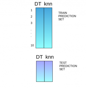
- This model is used to make final predictions on the test prediction set.
Sample code:
We first define a function to make predictions on n-folds of train and test dataset. This function returns the predictions for train and test for each model.
def Stacking(model,train,y,test,n_fold):
   folds=StratifiedKFold(n_splits=n_fold,random_state=1)
   test_pred=np.empty((test.shape[0],1),float)
   train_pred=np.empty((0,1),float)
   for train_indices,val_indices in folds.split(train,y.values):
      x_train,x_val=train.iloc[train_indices],train.iloc[val_indices]
      y_train,y_val=y.iloc[train_indices],y.iloc[val_indices]

      model.fit(X=x_train,y=y_train)
      train_pred=np.append(train_pred,model.predict(x_val))
      test_pred=np.append(test_pred,model.predict(test))
    return test_pred.reshape(-1,1),train_pred
Now we’ll create two base models – decision tree and knn.
model1 = tree.DecisionTreeClassifier(random_state=1)

test_pred1 ,train_pred1=Stacking(model=model1,n_fold=10, train=x_train,test=x_test,y=y_train)

train_pred1=pd.DataFrame(train_pred1)
test_pred1=pd.DataFrame(test_pred1)
model2 = KNeighborsClassifier()
test_pred2 ,train_pred2=Stacking(model=model2,n_fold=10,train=x_train,test=x_test,y=y_train)
train_pred2=pd.DataFrame(train_pred2)
test_pred2=pd.DataFrame(test_pred2)Create a third model, logistic regression, on the predictions of the decision tree and knn models.
df = pd.concat([train_pred1, train_pred2], axis=1)
df_test = pd.concat([test_pred1, test_pred2], axis=1)

model = LogisticRegression(random_state=1)
model.fit(df,y_train)
model.score(df_test, y_test)
In order to simplify the above explanation, the stacking model we have created has only two levels. The decision tree and knn models are built at level zero, while a logistic regression model is built at level one. Feel free to create multiple levels in a stacking model.
Blending
Blending follows the same approach as stacking but uses only a holdout (validation) set from the train set to make predictions. In other words, unlike stacking, the predictions are made on the holdout set only. The holdout set and the predictions are used to build a model which is run on the test set. Here is a detailed explanation of the blending process:
- The train set is split into training and validation sets.
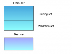
- Model(s) are fitted on the training set.
- The predictions are made on the validation set and the test set.
- The validation set and its predictions are used as features to build a new model.
- This model is used to make final predictions on the test and meta-features.
Sample Code:
We’ll build two models, decision tree and knn, on the train set in order to make predictions on the validation set.
model1 = tree.DecisionTreeClassifier()
model1.fit(x_train, y_train)
val_pred1=model1.predict(x_val)
test_pred1=model1.predict(x_test)
val_pred1=pd.DataFrame(val_pred1)
test_pred1=pd.DataFrame(test_pred1)

model2 = KNeighborsClassifier()
model2.fit(x_train,y_train)
val_pred2=model2.predict(x_val)
test_pred2=model2.predict(x_test)
val_pred2=pd.DataFrame(val_pred2)
test_pred2=pd.DataFrame(test_pred2)
Combining the meta-features and the validation set, a logistic regression model is built to make predictions on the test set.
df_val=pd.concat([x_val, val_pred1,val_pred2],axis=1)
df_test=pd.concat([x_test, test_pred1,test_pred2],axis=1)

model = LogisticRegression()
model.fit(df_val,y_val)
model.score(df_test,y_test)
Bagging
The idea behind bagging is combining the results of multiple models (for instance, all decision trees) to get a generalized result. Here’s a question: If you create all the models on the same set of data and combine it, will it be useful? There is a high chance that these models will give the same result since they are getting the same input. So how can we solve this problem? One of the techniques is bootstrapping.
Bootstrapping is a sampling technique in which we create subsets of observations from the original dataset, with replacement. The size of the subsets is the same as the size of the original set.
Bagging (or Bootstrap Aggregating) technique uses these subsets (bags) to get a fair idea of the distribution (complete set). The size of subsets created for bagging may be less than the original set.

- Multiple subsets are created from the original dataset, selecting observations with replacement.
- A base model (weak model) is created on each of these subsets.
- The models run in parallel and are independent of each other.

Boosting
Before we go further, here’s another question for you: If a data point is incorrectly predicted by the first model, and then the next (probably all models), will combining the predictions provide better results? Such situations are taken care of by boosting.
Boosting is a sequential process, where each subsequent model attempts to correct the errors of the previous model. The succeeding models are dependent on the previous model. Let’s understand the way boosting works in the below steps.
- A subset is created from the original dataset.
- Initially, all data points are given equal weights.
- A base model is created on this subset.
- This model is used to make predictions on the whole dataset.
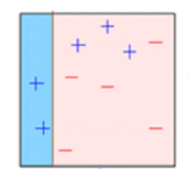
- Errors are calculated using the actual values and predicted values.
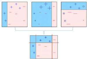
- The observations which are incorrectly predicted, are given higher weights.
(Here, the three misclassified blue-plus points will be given higher weights) - Another model is created and predictions are made on the dataset.
(This model tries to correct the errors from the previous model)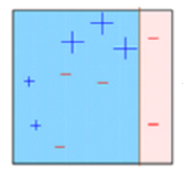
- Similarly, multiple models are created, each correcting the errors of the previous model.
- The final model (strong learner) is the weighted mean of all the models (weak learners).
 Thus, the boosting algorithm combines a number of weak learners to form a strong learner. The individual models would not perform well on the entire dataset, but they work well for some part of the dataset. Thus, each model actually boosts the performance of the ensemble.

Algorithms based on Bagging and Boosting
Bagging and Boosting are two of the most commonly used techniques in machine learning. In this section, we will look at them in detail. Following are the algorithms we will be focusing on:
Bagging algorithms:
- Bagging meta-estimator
- Random forest
Boosting algorithms:
- AdaBoost
- GBM
- XGBM
- Light GBM
- CatBoost
For all the algorithms discussed in this section, we will follow this procedure:
- Introduction to the algorithm
- Sample code
- Parameters
For this article, I have used the Loan Prediction Problem. You can download the dataset from here. Please note that a few code lines (reading the data, splitting into train-test sets, etc.) will be the same for each algorithm. In order to avoid repetition, I have written the code for the same below, and further discussed only the code for the algorithm.
#importing important packages
import pandas as pd
import numpy as np

#reading the dataset
df=pd.read_csv("/home/user/Desktop/train.csv")

#filling missing values
df['Gender'].fillna('Male', inplace=True)
Similarly, fill values for all the columns. EDA, missing values and outlier treatment has been skipped for the purposes of this article. To understand these topics, you can go through this article: Ultimate guide for Data Exploration in Python using NumPy, Matplotlib and Pandas.
#split dataset into train and test

from sklearn.model_selection import train_test_split
train, test = train_test_split(df, test_size=0.3, random_state=0)

x_train=train.drop('Loan_Status',axis=1)
y_train=train['Loan_Status']

x_test=test.drop('Loan_Status',axis=1)
y_test=test['Loan_Status']

#create dummies
x_train=pd.get_dummies(x_train)
x_test=pd.get_dummies(x_test)
Let’s jump into the bagging and boosting algorithms!
Bagging meta-estimator
Bagging meta-estimator is an ensembling algorithm that can be used for both classification (BaggingClassifier) and regression (BaggingRegressor) problems. It follows the typical bagging technique to make predictions. Following are the steps for the bagging meta-estimator algorithm:
- Random subsets are created from the original dataset (Bootstrapping).
- The subset of the dataset includes all features.
- A user-specified base estimator is fitted on each of these smaller sets.
- Predictions from each model are combined to get the final result.
Python Code
from sklearn.ensemble import BaggingClassifier
from sklearn import tree
model = BaggingClassifier(tree.DecisionTreeClassifier(random_state=1))
model.fit(x_train, y_train)
model.score(x_test,y_test)
0.75135135135135134
Sample code for regression problem
from sklearn.ensemble import BaggingRegressor
model = BaggingRegressor(tree.DecisionTreeRegressor(random_state=1))
model.fit(x_train, y_train)
model.score(x_test,y_test)
Parameters used in the algorithms
- base_estimator:
- It defines the base estimator to fit on random subsets of the dataset.
- When nothing is specified, the base estimator is a decision tree.
- n_estimators:
- It is the number of base estimators to be created.
- The number of estimators should be carefully tuned as a large number would take a very long time to run, while a very small number might not provide the best results.
- max_samples:
- This parameter controls the size of the subsets.
- It is the maximum number of samples to train each base estimator.
- max_features:
- Controls the number of features to draw from the whole dataset.
- It defines the maximum number of features required to train each base estimator.
- n_jobs:
- The number of jobs to run in parallel.
- Set this value equal to the cores in your system.
- If -1, the number of jobs is set to the number of cores.
- random_state:
- It specifies the method of random split. When random state value is same for two models, the random selection is same for both models.
- This parameter is useful when you want to compare different models.
Random Forest
Random Forest is another ensemble machine learning algorithm that follows the bagging technique. It is an extension of the bagging estimator algorithm. The base estimators in random forest are decision trees. Unlike bagging meta estimator, random forest randomly selects a set of features which are used to decide the best split at each node of the decision tree.
Looking at it step-by-step, this is what a random forest model does:
- Random subsets are created from the original dataset (bootstrapping).
- At each node in the decision tree, only a random set of features are considered to decide the best split.
- A decision tree model is fitted on each of the subsets.
- The final prediction is calculated by averaging the predictions from all decision trees.
Note: The decision trees in random forest can be built on a subset of data and features. Particularly, the sklearn model of random forest uses all features for decision tree and a subset of features are randomly selected for splitting at each node.
To sum up, Random forest randomly selects data points and features, and builds multiple trees (Forest).
Python Code:
Parameters
- n_estimators:
- It defines the number of decision trees to be created in a random forest.
- Generally, a higher number makes the predictions stronger and more stable, but a very large number can result in higher training time.
- criterion:
- It defines the function that is to be used for splitting.
- The function measures the quality of a split for each feature and chooses the best split.
- max_features :
- It defines the maximum number of features allowed for the split in each decision tree.
- Increasing max features usually improve performance but a very high number can decrease the diversity of each tree.
- max_depth:
- Random forest has multiple decision trees. This parameter defines the maximum depth of the trees.
- min_samples_split:
- Used to define the minimum number of samples required in a leaf node before a split is attempted.
- If the number of samples is less than the required number, the node is not split.
- min_samples_leaf:
- This defines the minimum number of samples required to be at a leaf node.
- Smaller leaf size makes the model more prone to capturing noise in train data.
- max_leaf_nodes:
- This parameter specifies the maximum number of leaf nodes for each tree.
- The tree stops splitting when the number of leaf nodes becomes equal to the max leaf node.
- n_jobs:
- This indicates the number of jobs to run in parallel.
- Set value to -1 if you want it to run on all cores in the system.
- random_state:
- This parameter is used to define the random selection.
- It is used for comparison between various models.
AdaBoost
Adaptive boosting or AdaBoost is one of the simplest boosting algorithms. Usually, decision trees are used for modelling. Multiple sequential models are created, each correcting the errors from the last model. AdaBoost assigns weights to the observations that are incorrectly predicted, and the subsequent model works to predict these values correctly.
Below are the steps for performing the AdaBoost algorithm:
- Initially, all observations in the dataset are given equal weights.
- A model is built on a subset of data.
- Using this model, predictions are made on the whole dataset.
- Errors are calculated by comparing the predictions and actual values.
- While creating the next model, higher weights are given to the data points which were predicted incorrectly.
- Weights can be determined using the error value. For instance, higher the error more is the weight assigned to the observation.
- This process is repeated until the error function does not change, or the maximum limit of the number of estimators is reached.
Python Code
from sklearn.ensemble import AdaBoostClassifier
model = AdaBoostClassifier(random_state=1)
model.fit(x_train, y_train)
model.score(x_test,y_test)
0.81081081081081086
Sample code for regression problem
from sklearn.ensemble import AdaBoostRegressor
model = AdaBoostRegressor()
model.fit(x_train, y_train)
model.score(x_test,y_test)
Parameters
- base_estimators:
- It helps to specify the type of base estimator, that is, the machine learning algorithm to be used as base learner.
- n_estimators:
- It defines the number of base estimators.
- The default value is 10, but you should keep a higher value to get better performance.
- learning_rate:
- This parameter controls the contribution of the estimators in the final combination.
- There is a trade-off between learning_rate and n_estimators.
- max_depth:
- Defines the maximum depth of the individual estimator.
- Tune this parameter for best performance.
- n_jobs
- Specifies the number of processors it is allowed to use.
- Set value to -1 for maximum processors allowed.
- random_state :
- An integer value to specify the random data split.
- A definite value of random_state will always produce same results if given with same parameters and training data.
Gradient Boosting (GBM)
Gradient Boosting or GBM is another ensemble machine learning algorithm that works for both regression and classification problems. GBM uses the boosting technique, combining a number of weak learners to form a strong learner. Regression trees used as a base learner, each subsequent tree in series is built on the errors calculated by the previous tree.
We will use a simple example to understand the GBM algorithm. We have to predict the age of a group of people using the below data:

- The mean age is assumed to be the predicted value for all observations in the dataset.
- The errors are calculated using this mean prediction and actual values of age.

- A tree model is created using the errors calculated above as target variable. Our objective is to find the best split to minimize the error.
- The predictions by this model are combined with the predictions 1.

- This value calculated above is the new prediction.
- New errors are calculated using this predicted value and actual value.

- Steps 2 to 6 are repeated till the maximum number of iterations is reached (or error function does not change).
Python Code
from sklearn.ensemble import GradientBoostingClassifier
model= GradientBoostingClassifier(learning_rate=0.01,random_state=1)
model.fit(x_train, y_train)
model.score(x_test,y_test)
0.81621621621621621
Sample code for regression problem
from sklearn.ensemble import GradientBoostingRegressor
model= GradientBoostingRegressor()
model.fit(x_train, y_train)
model.score(x_test,y_test)
Parameters
- min_samples_split
- Defines the minimum number of samples (or observations) which are required in a node to be considered for splitting.
- Used to control over-fitting. Higher values prevent a model from learning relations which might be highly specific to the particular sample selected for a tree.
- min_samples_leaf
- Defines the minimum samples required in a terminal or leaf node.
- Generally, lower values should be chosen for imbalanced class problems because the regions in which the minority class will be in the majority will be very small.
- min_weight_fraction_leaf
- Similar to min_samples_leaf but defined as a fraction of the total number of observations instead of an integer.
- max_depth
- The maximum depth of a tree.
- Used to control over-fitting as higher depth will allow the model to learn relations very specific to a particular sample.
- Should be tuned using CV.
- max_leaf_nodes
- The maximum number of terminal nodes or leaves in a tree.
- It can define max_depth. Since binary trees are created, a depth of ‘n’ would produce a maximum of 2^n leaves.
- If this is defined, GBM will ignore max_depth.
- max_features
- The number of features to consider while searching for the best split. These will be randomly selected.
- As a thumb-rule, the square root of the total number of features works great but we should check up to 30-40% of the total number of features.
- Higher values can lead to over-fitting but it generally depends on a case to case scenario.
XGBoost
XGBoost (extreme Gradient Boosting) is an advanced implementation of the gradient boosting algorithm. It has proved to be a highly effective ML algorithm, extensively used in machine learning competitions and hackathons. XGBoost has high predictive power and is almost 10 times faster than the other gradient boosting techniques. It also includes a variety of regularization which reduces overfitting and improves overall performance. Hence it is also known as ‘regularized boosting‘ technique.
Let us see how XGBoost is comparatively better than other techniques:
- Regularization:
- Standard GBM implementation has no regularisation like XGBoost.
- Thus XGBoost also helps to reduce overfitting.
- Parallel Processing:
- XGBoost implements parallel processing and is faster than GBM .
- XGBoost also supports implementation on Hadoop.
- High Flexibility:
- XGBoost allows users to define custom optimization objectives and evaluation criteria adding a whole new dimension to the model.
- Handling Missing Values:
- XGBoost has an in-built routine to handle missing values.
- Tree Pruning:
- XGBoost makes splits up to the max_depth specified and then starts pruning the tree backwards and removes splits beyond which there is no positive gain.
- Built-in Cross-Validation:
- XGBoost allows a user to run a cross-validation at each iteration of the boosting process and thus it is easy to get the exact optimum number of boosting iterations in a single run.
Python Code
Since XGBoost takes care of the missing values itself, you do not have to impute the missing values. You can skip the step for missing value imputation from the code mentioned above. Follow the remaining steps as always and then apply xgboost as below.
import xgboost as xgb
model=xgb.XGBClassifier(random_state=1,learning_rate=0.01)
model.fit(x_train, y_train)
model.score(x_test,y_test)
0.82702702702702702
Sample code for regression problem
import xgboost as xgb
model=xgb.XGBRegressor()
model.fit(x_train, y_train)
model.score(x_test,y_test)
Parameters
- nthread
- This is used for parallel processing and the number of cores in the system should be entered..
- If you wish to run on all cores, do not input this value. The algorithm will detect it automatically.
- eta
- Analogous to learning rate in GBM.
- Makes the model more robust by shrinking the weights on each step.
- min_child_weight
- Defines the minimum sum of weights of all observations required in a child.
- Used to control over-fitting. Higher values prevent a model from learning relations which might be highly specific to the particular sample selected for a tree.
- max_depth
- It is used to define the maximum depth.
- Higher depth will allow the model to learn relations very specific to a particular sample.
- max_leaf_nodes
- The maximum number of terminal nodes or leaves in a tree.
- Can be defined in place of max_depth. Since binary trees are created, a depth of ‘n’ would produce a maximum of 2^n leaves.
- If this is defined, GBM will ignore max_depth.
- gamma
- A node is split only when the resulting split gives a positive reduction in the loss function. Gamma specifies the minimum loss reduction required to make a split.
- Makes the algorithm conservative. The values can vary depending on the loss function and should be tuned.
- subsample
- Same as the subsample of GBM. Denotes the fraction of observations to be randomly sampled for each tree.
- Lower values make the algorithm more conservative and prevent overfitting but values that are too small might lead to under-fitting.
- colsample_bytree
- It is similar to max_features in GBM.
- Denotes the fraction of columns to be randomly sampled for each tree.
Light GBM
Before discussing how Light GBM works, let’s first understand why we need this algorithm when we have so many others (like the ones we have seen above). Light GBM beats all the other algorithms when the dataset is extremely large. Compared to the other algorithms, Light GBM takes lesser time to run on a huge dataset.
LightGBM is a gradient boosting framework that uses tree-based algorithms and follows leaf-wise approach while other algorithms work in a level-wise approach pattern. The images below will help you understand the difference in a better way.


Leaf-wise growth may cause over-fitting on smaller datasets but that can be avoided by using the ‘max_depth’ parameter for learning. You can read more about Light GBM and its comparison with XGB in this article.
Python Code
import lightgbm as lgb
train_data=lgb.Dataset(x_train,label=y_train)
#define parameters
params = {'learning_rate':0.001}
model= lgb.train(params, train_data, 100)
y_pred=model.predict(x_test)
for i in range(0,185):
   if y_pred[i]>=0.5:
   y_pred[i]=1
else:
   y_pred[i]=0
0.81621621621621621
Sample code for regression problem
import lightgbm as lgb
train_data=lgb.Dataset(x_train,label=y_train)
params = {'learning_rate':0.001}
model= lgb.train(params, train_data, 100)
from sklearn.metrics import mean_squared_error
rmse=mean_squared_error(y_pred,y_test)**0.5
Parameters
- num_iterations:
- It specifies the number of boosting iterations to perform.
- num_leaves :
- This parameter sets the number of leaves to form in a tree.
- In case of Light GBM, since splitting takes place leaf-wise rather than depth-wise, num_leaves must be smaller than 2^(max_depth), otherwise, it may lead to overfitting.
- min_data_in_leaf :
- A very small value may cause overfitting.
- It is also one of the most important parameters in dealing with overfitting.
- max_depth:
- It specifies the maximum depth or level up to which a tree can grow.
- A very high value for this parameter can cause overfitting.
- bagging_fraction:
- It specifies the fraction of data to use for each iteration.
- This parameter generally speeds up the training.
- max_bin :
- It defines the maximum number of bins that feature values will be bucketed into.
- A smaller value of max_bin can save a lot of time as it buckets the feature values in discrete bins which is computationally inexpensive.
CatBoost
Handling categorical variables is a tedious process, especially when you have a large number of such variables. When your categorical variables have too many labels (i.e. they are highly cardinal), performing one-hot-encoding on them exponentially increases the dimensionality and it becomes really difficult to work with the dataset.
CatBoost can automatically deal with categorical variables and does not require extensive data preprocessing like other machine learning algorithms. Here is an article that explains CatBoost in detail.
Python Code
CatBoost algorithm effectively deals with categorical variables. Thus, you should not perform one-hot encoding for categorical variables. Just load the files, impute missing values, and you’re good to go.
from catboost import CatBoostClassifier
model=CatBoostClassifier()
categorical_features_indices = np.where(df.dtypes != np.float)[0]
model.fit(x_train,y_train,cat_features=([ 0,  1, 2, 3, 4, 10]),eval_set=(x_test, y_test))
model.score(x_test,y_test)
0.80540540540540539
Sample code for regression problem
from catboost import CatBoostRegressor
model=CatBoostRegressor()
categorical_features_indices = np.where(df.dtypes != np.float)[0]
model.fit(x_train,y_train,cat_features=([ 0,  1, 2, 3, 4, 10]),eval_set=(x_test, y_test))
model.score(x_test,y_test)
Parameters
- loss_function:
- Defines the metric to be used for training.
- iterations:
- The maximum number of trees that can be built.
- The final number of trees may be less than or equal to this number.
- learning_rate:
- Defines the learning rate.
- Used for reducing the gradient step.
- border_count:
- It specifies the number of splits for numerical features.
- It is similar to the max_bin parameter.
- depth:
- Defines the depth of the trees.
- random_seed:
- This parameter is similar to the ‘random_state’ parameter we have seen previously.
- It is an integer value to define the random seed for training.
This brings us to the end of the ensemble algorithms section. We have covered quite a lot in this article!
Conclusion
Ensemble modeling can exponentially boost the performance of your model and can sometimes be the deciding factor between first place and second! In this article, we covered various ensemble learning techniques and saw how these techniques are applied in machine learning algorithms. Further, we implemented the algorithms on our loan prediction dataset.
This article will have given you a solid understanding of this topic. If you have any suggestions or questions, do share in the comment section below. Also, I encourage you to implement these algorithms at your end and share your results with us!
And if you want to hone your skills as a data science professional then I will recommend you take up this comprehensive course that provides you all the tools and techniques you need to apply machine learning to solve business problems.
Frequently Asked Questions
Q1. What is bagging and boosting in machine learning?
A. Bagging and boosting are ensemble learning techniques in machine learning. Bagging trains multiple models on different subsets of training data with replacement and combines their predictions to reduce variance and improve generalization. Boosting combines multiple weak learners to create a strong learner by focusing on misclassified data points and assigning higher weights in the next iteration. Examples of bagging algorithms include Random Forest while boosting algorithms include AdaBoost, Gradient Boosting, and XGBoost.
Q2. What is difference between bagging and boosting?
A. Bagging reduces variance by training multiple models independently on different subsets of training data and combining their predictions, while boosting reduces bias by iteratively training weak learners and focusing on misclassified data points to create a strong learner. Random Forest is a popular bagging algorithm, while AdaBoost, Gradient Boosting, and XGBoost are popular boosting algorithms.
Q3. Which are the three types of ensemble learning?
1. Bagging: Creates multiple models from different training data samples, reducing variance.
2. Boosting: Creates multiple models with weighted training data, reducing bias.
3. Stacking: Combines predictions of multiple models using a meta-model, enhancing generalization.
The media shown in this article is not owned by Analytics Vidhya and is used at the Author’s discretion.
AdaBoostaveragingbaggingblendingBoostingensemble learningGBMlight gbmlive codingmax votingrandom foreststackingweighted averagingxgb
Aishwarya Singh
24 May, 2024
An avid reader and blogger who loves exploring the endless world of data science and artificial intelligence. Fascinated by the limitless applications of ML and AI; eager to learn and discover the depths of data science.


Really nice article! And just when I needed the most. Could you please upload the dataset you used? Im having an error regarding the shapes when implementing the Stacking Ensemble. Thank you!
Hi Joaquin, Glad you found this useful. You can download the dataset from this link.
Nice Article !!!
Thanks Aditya
Thank you. This is great content. Been following it from the beginning. 2 issues: Getting NameError: tree is not defined. Secondly, from section 4 onwards, there is dataset to work on. But no dataset referred to for sections before 4. So cannot run the code on data. NameError Traceback (most recent call last) in () 3 from sklearn.ensemble import BaggingClassifier 4 #model = tree.DecisionTreeClassifier() ----> 5 model = BaggingClassifier(tree.DecisionTreeClassifier(random_state=1)) 6 model.fit(x_train, y_train) 7 model.score(x_test,y_test) NameError: name 'tree' is not defined For beginners like me, will need a little more detail to follow the full notebook.
Hi Sanjoy, The codes for voting and averaging can be used with any dataset, and hence no particular dataset is attached to that section. You can try implementing the codes on loan prediction dataset and if you face any issues do let me know. Regarding the error 'tree not found' , please use the following code line : from sklearn import tree. Thank you for pointing it out. I will update the same in the post.
Wonderful article
Thank you
Hi, In section 3.3 bagging at one point you mentioned that "The size of the subsets is the same as the size of the original set." when you are explaining bootstraping and in the next paragraph you are saying "The size of subsets created for bagging may be less than the original set." Please make it clear. Nice Article !!
Hi Abhinav, In bootstrapping, the size of subsets are same as the size of the original set. While in bagging, the size of each subset may be equal to or lesser than the size of the original set.
kindly explain the same using R language
Hi meharunnisa, Here is an article on ensemble learning in R : How to build Ensemble Models in machine learning? (with code in R)
Can you please explain how did you calculate the Prediction 2 in gradient boosting?
Hi Ishit, In this case, I have taken a simple example to explain the concept. So the residuals are considered as target for next decision tree. The decision tree splits such that the similar target are in the same node. Further the average of the node is calculated. This is assigned to all the values in the as new predictions. I have made some update, please check if it clarifies your doubt now. If you still face any issue, do let me know.
Thanks for the article, Aishwarya!
Hi Ajay, Glad you liked it!
Hi Aishwarya, Do you have any contact information that you can share with me? I would like to speak to you about a possible career opportunity. Thanks, Nitin Gupta VP | Product Architect @ Dori Inc.
Can you please explain how did you calculate the Prediction 2 in gradient boosting? For Prediction 1 you use following method mean age =combine all age / number of person age Residual 1 = age - mean age in same way how you have calculated predication 2
Hi, We create a decision tree on the residuals. Let us suppose that the decision tree splits such that all positive numbers are in one leaf node while negative in other (Just an example, the results are much more complicated). The average for each leaf node is taken as the predicted value. Further these values are combined with the mean and new residuals are created.
Thank you for a very informative article. Just one issue: When fitting the BaggingRegressor to the training data, I get the following error: ValueError: could not convert string to float: 'Y' I'm assuming it's because we need to convert the y_train to {1,0} Am I correct? Thanks much Jorge
Hi Jorge, If your target variable is 'Y' and 'N' , you should use BaggingClassifier instead of BaggingRegressor.
Great article. Keep up the good work !
Thank you
This is very nice, Hoe do you see this in Prod ? Anyway great work.
A nice article But if i need to use boosting or bagging using different models like (decision tree, random forest, logistic regression ) how can i implement it ?
Hi Aymen, If you see the code for bagging classifier, you will observe that we can provide the classifier we wish to use. As an example, I have used decision tree, you can use random forest or logistic regression.
Hi !, in the stacking function, you are initiating "test_pred" with some random floats of shape (test.shape[0],1) code: test_pred = np.empty(test.shape[0],1,float) later in the same function , you are appending the predicted values of "test" dataset to the already existing "test_pred"., 1) if "test_pred" is the predictions of the "test" dataset that we pass in the funciton, they should have same number of rows, but in the way it was coded, the number of rows will be twice the number of rows of "test" dataset, since "test_pred" was already initiated with some random numbers(the empty commad generates) of rows equal to rows in "test", and then adding the equal number of additional predictions to those already existing rows(while appending the predicitons of test), need some clarification... ex: in example show, the shape of "test_pred" should be (154,1) since "test" dataset passed was of shape(154,8)., but the shape the function "test_pred" the function is returning is twice ie., (308,1) 2) And any particular reason, why "test_pred" was not initiated like "train_pred" with empty array shape (0,1), instead of shape (test.shape[0],1) ?
Hi manoj, When I use np.empty(shape), it should give me an empty array of the shape assigned. If you are getting an error, replace this line and define test_pred in the same way as train_pred is defined.
Hello Manoj, I think `test_pred=np.append(test_pred,model.predict(test))` should be placed outside the for loop.
Thanks for this awesome post. Do you hav any posts explaining stacked ensemble of pretrained Deep Learning models with image inputs? Can you point to any resources otherwise?
Hi Shiva, I haven't researched on ensemble of pretrained models yet. If I come across a relevant post, I'd share it with you.
Hey thanks very much for your help. I am trying to run the stacking method and I got this error AttributeError: 'numpy.ndarray' object has no attribute 'values'. Can you please explain me why. Pd. I am new on programming :D Thanks in advance
Hi, Looks like the you are using
.valueson an array. Convert it into a dataframe and use the command.How should I miss such a great article before??? I have become your fan now, AISHWARYA!!! Love "Concept + Code" blog, easy to follow and implement. Appreciate your time !!!
Thanks a lot!
The stacking simple code ,I cant pass,i raise error when socre model --------------------------------------------------------------------------- ValueError Traceback (most recent call last) in () 4 model = LogisticRegression(random_state=1) 5 model.fit(df,y_train) ----> 6 model.score(df_test, y_test) E:\ProgramData\Anaconda3\lib\site-packages\sklearn\base.py in score(self, X, y, sample_weight) 347 """ 348 from .metrics import accuracy_score --> 349 return accuracy_score(y, self.predict(X), sample_weight=sample_weight) 350 351 E:\ProgramData\Anaconda3\lib\site-packages\sklearn\metrics\classification.py in accuracy_score(y_true, y_pred, normalize, sample_weight) 174 175 # Compute accuracy for each possible representation --> 176 y_type, y_true, y_pred = _check_targets(y_true, y_pred) 177 if y_type.startswith('multilabel'): 178 differing_labels = count_nonzero(y_true - y_pred, axis=1) E:\ProgramData\Anaconda3\lib\site-packages\sklearn\metrics\classification.py in _check_targets(y_true, y_pred) 69 y_pred : array or indicator matrix 70 """ ---> 71 check_consistent_length(y_true, y_pred) 72 type_true = type_of_target(y_true) 73 type_pred = type_of_target(y_pred) E:\ProgramData\Anaconda3\lib\site-packages\sklearn\utils\validation.py in check_consistent_length(*arrays) 202 if len(uniques) > 1: 203 raise ValueError("Found input variables with inconsistent numbers of" --> 204 " samples: %r" % [int(l) for l in lengths]) 205 206 ValueError: Found input variables with inconsistent numbers of samples: [192, 2112]
Thanks for the detailed and organized article. Could you please help me on following issue? df has 2 features and we fitted the level one model to df and y_train, my question is how can we use this model to predict x_test as we need to get y_test (predicted y for test data set) for x_test. Model fitted with 2 features but x_test has 20 features so could not use the model for x_test. For example if I want to use level one model to predict Loan_Status for Loan Prediction competition after(model.fit(df,y_train)) how can I use model.predict(x_test)? Showing following error.! ValueError: X has 20 features per sample; expecting 2
Hi Sadiq, The dataset you train and the daatset on which you want to predict should have the same number of features. df should have 20 features or you will have to drop the remaining 18 features from x_test. Which part of the code in the article (or uder which section) did you face the error?
same issue i have error like this ; ValueError: Found array with dim 4. Estimator expected <= 2. how to solved this ?
Well organized and informative article. I have a question: What do you think about their usage in real life. Although there are powerful boosting algoritms( like "XGBoost"), do we still need stacking, blending or voting based learning? Thank you
Hi, I am aware that we have powerful algorithms that are able to give excellent performance. But the idea behind covering the concepts of stacking, blending was to start with the basics and then move to complex algorithms
It is a very useful article for ensemble methods. But while using blending, I get the error "cannot concatenate a non-NDFrame object. Can you please guide me to avoid the error?
Hi shukrity, Please check the type of the data you are using. is it a dataframe?
Nice article. However, I am looking for ensemble for Keras model. Can you share your knowledge please?
Can you please help me out of my problem regarding stacking. In my dataset, size of train set is 7116 and size of test set is 1780. So, df_test and y_test should same in size(1780). But, size of df_test is shown 10680. So,value error arises for this inconsistency. Please tell me how can I solve this problem?
Could you share the notebook with me? Or the code so that I can copy paste and check at my end.
Nice Article !!!
Hi Aishwarya, thanks for this prefect post ,, i want ask you , I'm tying to do stacking deep learning with ptrained models, i trined the models on train set then build new model his input are the first level models output and train the new models on new dataset, at the end i evaluated all models on the same test det of the first dataset ... i got better resuls ,,, Is this right? can i called this way stacking? or what? thank in advance ^-^
Excellent compilation with ease of understanding the core subject. Well explained all the methods in one place . Thanks for nice sharing .
Well explained. Thank you.