XGBoost is a machine learning algorithm that belongs to the ensemble learning category, specifically the gradient boosting framework. It utilizes decision trees as base learners and employs regularization techniques to enhance model generalization. XGBoost is famous for its computational efficiency, offering efficient processing, insightful feature importance analysis, and seamless handling of missing values. It’s the go-to algorithm for a wide range of tasks, including regression, classification, and ranking. In this article, we will give you an overview of XGBoost model, along with a use-case!
We recommend going through the below article as well to fully understand the various terms and concepts mentioned in this article:
XGBoost, or eXtreme Gradient Boosting, is a XGBoost algorithm in machine learning algorithm under ensemble learning. It is trendy for supervised learning tasks, such as regression and classification. XGBoost builds a predictive model by combining the predictions of multiple individual models, often decision trees, in an iterative manner.
The algorithm works by sequentially adding weak learners to the ensemble, with each new learner focusing on correcting the errors made by the existing ones. It uses a gradient descent optimization technique to minimize a predefined loss function during training.
Key features of XGBoost Algorithm include its ability to handle complex relationships in data, regularization techniques to prevent overfitting and incorporation of parallel processing for efficient computation.
XGBoost is an ensemble learning method. Sometimes, it may not be sufficient to rely upon the results of just one machine learning model. Ensemble learning offers a systematic solution to combine the predictive power of multiple learners. The resultant is a single model which gives the aggregated output from several models.
The models that form the ensemble, also known as base learners, could be either from the same learning algorithm or different learning algorithms. Bagging and boosting are two widely used ensemble learners. Though these two techniques can be used with several statistical models, the most predominant usage has been with decision trees.
Let’s briefly discuss bagging before taking a more detailed look at the concept of gradient boosting.
While decision trees are one of the most easily interpretable models, they exhibit highly variable behavior. Consider a single training dataset that we randomly split into two parts. Now, let’s use each part to train a decision tree in order to obtain two models.
When we fit both these models, they would yield different results. Decision trees are said to be associated with high variance due to this behavior. Bagging or boosting aggregation helps to reduce the variance in any learner. Several decision trees which are generated in parallel, form the base learners of bagging technique. Data sampled with replacement is fed to these learners for training. The final prediction is the averaged output from all the learners.
In boosting, the trees are built sequentially such that each subsequent tree aims to reduce the errors of the previous tree. Each tree learns from its predecessors and updates the residual errors. Hence, the tree that grows next in the sequence will learn from an updated version of the residuals.
The base learners in boosting are weak learners in which the bias is high, and the predictive power is just a tad better than random guessing. Each of these weak learners contributes some vital information for prediction, enabling the boosting technique to produce a strong learner by effectively combining these weak learners. The final strong learner brings down both the bias and the variance.
In contrast to bagging techniques like Random Forest, in which trees are grown to their maximum extent, boosting makes use of trees with fewer splits. Such small trees, which are not very deep, are highly interpretable. Parameters like the number of trees or iterations, the rate at which the gradient boosting learns, and the depth of the tree, could be optimally selected through validation techniques like k-fold cross validation. Having a large number of trees might lead to overfitting. So, it is necessary to carefully choose the stopping criteria for boosting.
The gradient boosting ensemble technique consists of three simple steps:
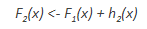
To improve the performance of F1, we could model after the residuals of F1 and create a new model F2:
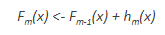
This can be done for ‘m’ iterations, until residuals have been minimized as much as possible:
Here, the additive learners do not disturb the functions created in the previous steps. Instead, they impart information of their own to bring down the errors.
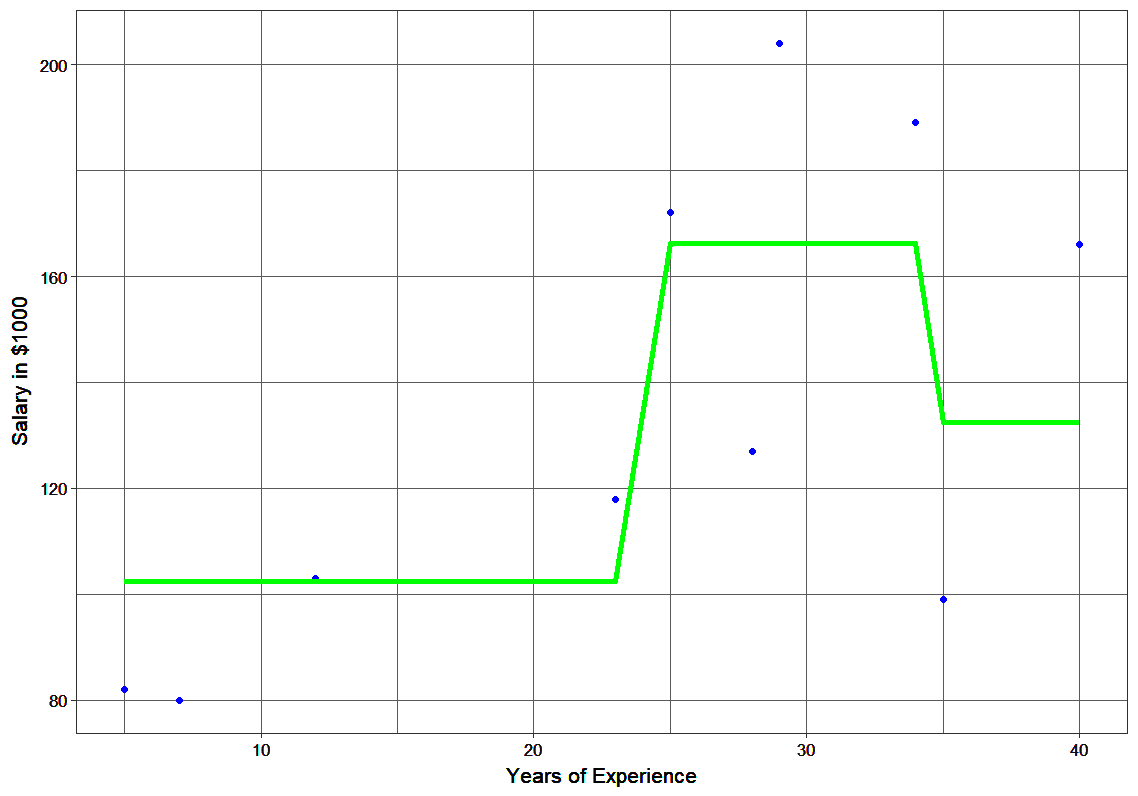
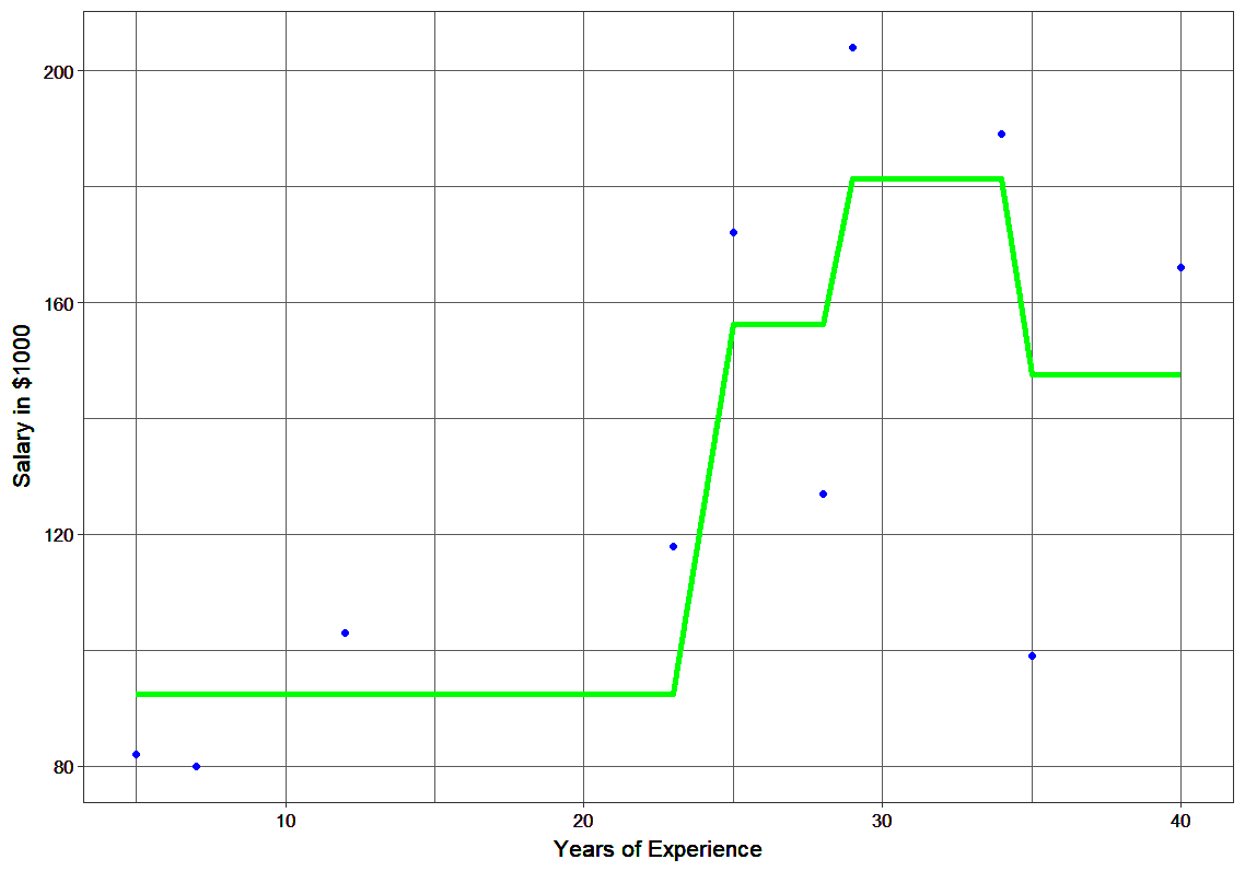
In this section, we will explore the power of gradient boosting, a machine learning technique, by building an ensemble model to predict salary based on years of experience. By utilizing regression trees and optimizing loss functions, we aim to showcase the significant reduction in error that gradient boosting can achieve.
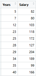
Consider the following data where the years of experience is predictor variable and salary (in thousand dollars) is the target. Using regression trees as base learners, we can create an ensemble model to predict the salary. For the sake of simplicity, we can choose square loss as our loss function and our objective would be to minimize the square error.
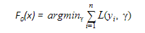
As the first step, the model should be initialized with a function F0(x). F0(x) should be a function which minimizes the loss function or MSE (mean squared error), in this case:

Taking the first differential of the above equation with respect to γ, it is seen that the function minimizes at the mean i=1nyin. So, the boosting model could be initiated with:

F0(x) gives the predictions from the first stage of our model. Now, the residual error for each instance is (yi – F0(x)).
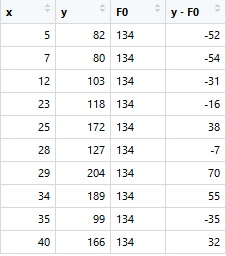
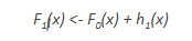
We can use the residuals from F0(x) to create h1(x). h1(x) will be a regression tree which will try and reduce the residuals from the previous step. The output of h1(x) won’t be a prediction of y; instead, it will help in predicting the successive function F1(x) which will bring down the residuals.
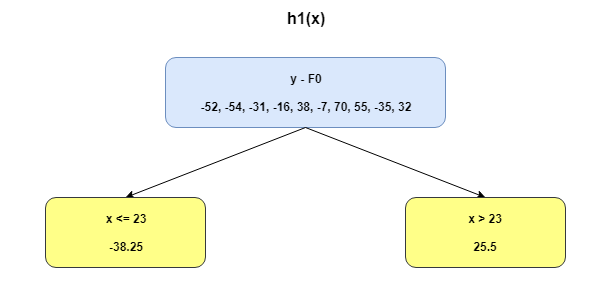
The additive model h1(x) computes the mean of the residuals (y – F0) at each leaf of the tree. The boosted function F1(x) is obtained by summing F0(x) and h1(x). This way h1(x) learns from the residuals of F0(x) and suppresses it in F1(x).

This can be repeated for 2 more iterations to compute h2(x) and h3(x). Each of these additive learners, hm(x), will make use of the residuals from the preceding function, Fm-1(x).
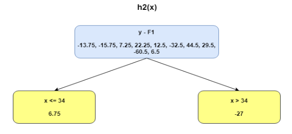
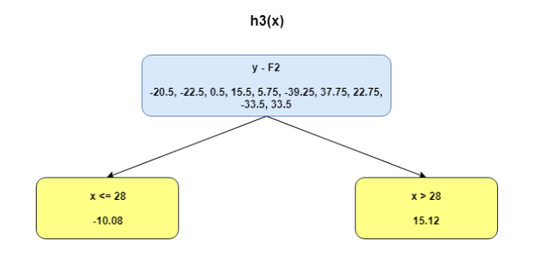
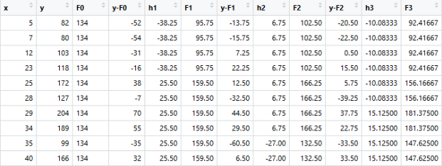
The MSEs for F0(x), F1(x) and F2(x) are 875, 692 and 540. It’s amazing how these simple weak learners can bring about a huge reduction in error!
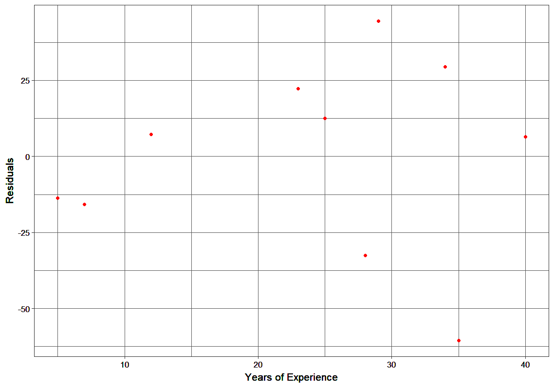
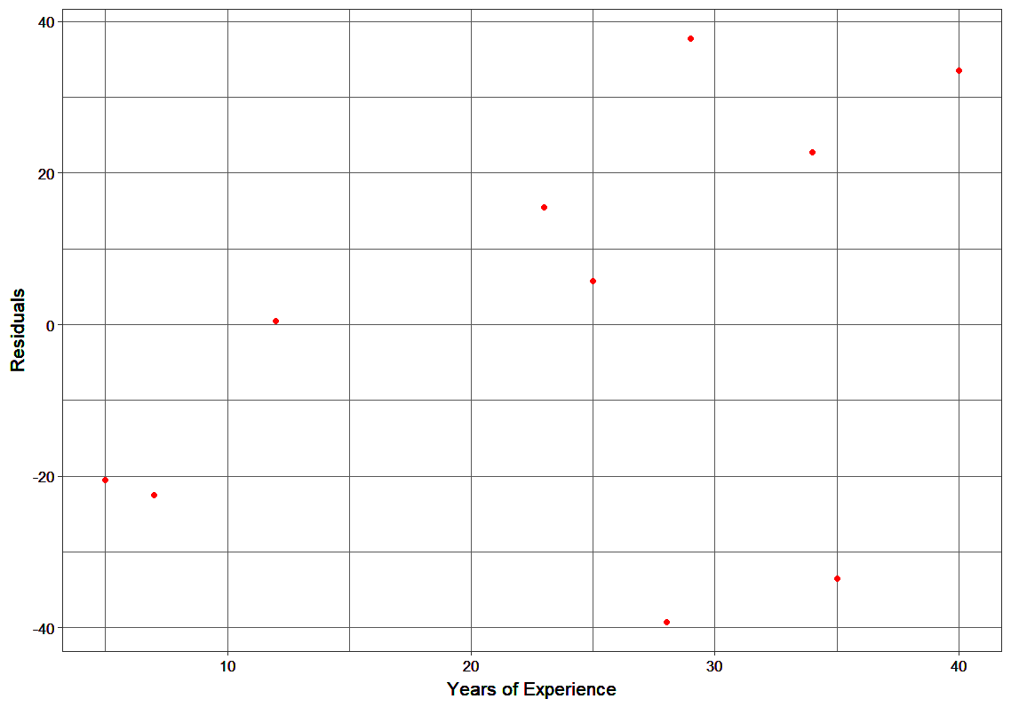
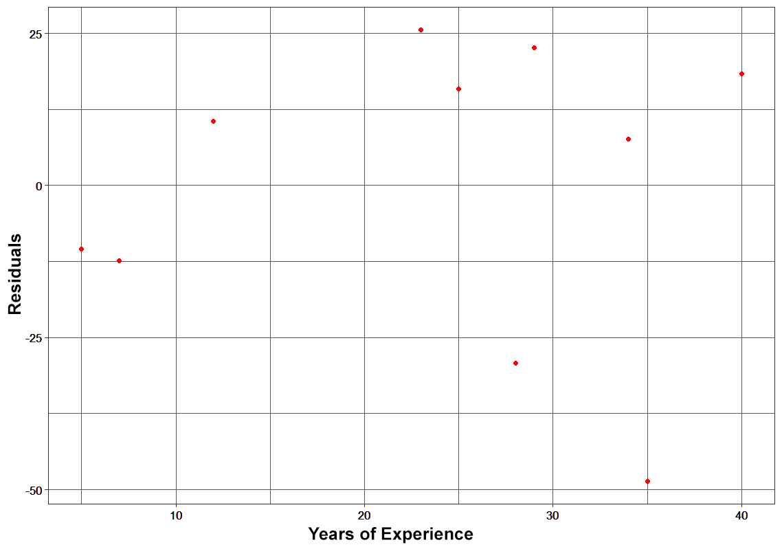
Note that each learner, hm(x), is trained on the residuals. All the additive learners in boosting are modeled after the residual errors at each step. Intuitively, it could be observed that the boosting learners make use of the patterns in residual errors. At the stage where maximum accuracy is reached by boosting, the residuals appear to be randomly distributed without any pattern.

In the case discussed above, MSE was the loss function. The mean minimized the error here. When MAE (mean absolute error) is the loss function, the median would be used as F₀(x) to initialize the model. A unit change in y would cause a unit change in MAE as well. Using scikit-learn, you can implement various models, including tree boosting algorithms and linear regression models to analyze the differences in loss functions and their impact on the model’s performance.
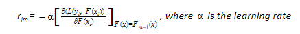
For MSE, the change observed would be roughly exponential. Instead of fitting hm(x) on the residuals, fitting it on the gradient of loss function, or the step along which loss occurs, would make this process generic and applicable across all loss functions.
Gradient descent helps us minimize any differentiable function. Earlier, the regression tree for hm(x) predicted the mean residual at each terminal node of the tree. In gradient boosting, the average gradient component would be computed.
For each node, there is a factor γ with which hm(x) is multiplied. This accounts for the difference in impact of each branch of the split. Gradient boosting helps in predicting the optimal gradient for the additive model, unlike classical gradient descent techniques which reduce error in the output at each iteration.
The following steps are involved in gradient boosting:

XGBoost model is a popular implementation of gradient boosting. Let’s discuss some features or metrics of XGBoost that make it so interesting:
Here’s a live coding window to see how XGBoost works and play around with the code without leaving this article!
'''
The following code is for XGBoost
Created by - ANALYTICS VIDHYA
'''

# importing required libraries
import pandas as pd
from xgboost import XGBClassifier
from sklearn.metrics import accuracy_score

# read the train and test dataset
train_data = pd.read_csv('train-data.csv')
test_data = pd.read_csv('test-data.csv')

# shape of the dataset
print('Shape of training data :',train_data.shape)
print('Shape of testing data :',test_data.shape)

# Now, we need to predict the missing target variable in the test data
# target variable - Survived

# seperate the independent and target variable on training data
train_x = train_data.drop(columns=['Survived'],axis=1)
train_y = train_data['Survived']

# seperate the independent and target variable on testing data
test_x = test_data.drop(columns=['Survived'],axis=1)
test_y = test_data['Survived']

'''
Create the object of the XGBoost model
You can also add other parameters and test your code here
Some parameters are : max_depth and n_estimators
Documentation of xgboost:

https://xgboost.readthedocs.io/en/latest/
'''
model = XGBClassifier()

# fit the model with the training data
model.fit(train_x,train_y)


# predict the target on the train dataset
predict_train = model.predict(train_x)
print('\nTarget on train data',predict_train)

# Accuray Score on train dataset
accuracy_train = accuracy_score(train_y,predict_train)
print('\naccuracy_score on train dataset : ', accuracy_train)

# predict the target on the test dataset
predict_test = model.predict(test_x)
print('\nTarget on test data',predict_test)

# Accuracy Score on test dataset
accuracy_test = accuracy_score(test_y,predict_test)
print('\naccuracy_score on test dataset : ', accuracy_test)| Feature | XGBoost | Gradient Boosting |
|---|---|---|
| Description | Advanced implementation of gradient boosting | Ensemble technique using weak learners |
| Optimization | Regularized objective function | Error gradient minimization |
| Efficiency | Highly optimized, efficient | Computationally intensive |
| Missing Values | Built-in support | Requires preprocessing |
| Regularization | Built-in L1 and L2 | Requires external steps |
| Feature Importance | Built-in measures | Limited, needs external calculation |
| Interpretability | Complex, less interpretable | More interpretable models |
| Feature | XGBoost | Random Forest |
|---|---|---|
| Description | Improves mistakes from previous trees | Builds trees independently |
| Algorithm Type | Boosting | Bagging |
| Handling of Weak Learners | Corrects errors sequentially | Combines predictions of independently built trees |
| Regularization | Uses L1 and L2 regularization to prevent overfitting | Usually doesn’t employ regularization techniques |
| Performance | Often performs better on structured data but needs more tuning | Simpler and less prone to overfitting |
So that was all about the mathematics that power the popular XGBoost algorithm. If your basics are solid, this article must have been a breeze for you. It’s such a powerful algorithm and while there are other techniques that have spawned from it (like CATBoost), XGBoost Model remains a game changer in the machine learning community. We highly recommend you to take up this course to sharpen your skills in machine learning and learn all the state-of-the-art techniques used in the field with our Applied Machine Learning – Beginner to Professional course. Also, these Algorithm helps you for training data. and help you for learning rate that will help you for lightgbm the algorithms.
A. The performance of XGBoost and random forest depends on the data and problem being solved. XGBoost tends to perform better on structured data, while random forest can be more effective on unstructured data.
A. XGBoost Python is a Python package that enables building and training models using the XGBoost algorithm in Python. It includes many functions for tuning and optimizing model performance.
A. XGBoost is a versatile algorithm, applicable to both classification and regression tasks. It effectively manages various data types and can be tailored to meet specific requirements.
XGBoost is an AI tool. It’s a machine learning algorithm that helps AI systems make better predictions. You can also see it in github and kaggle.
XGBoost Classifier is a gradient boosting classifier. It’s a kind of ensemble classifier that improves by learning from past mistakes, often used for structured data tasks.
Lorem ipsum dolor sit amet, consectetur adipiscing elit,


Nice explanation !
Hi. Nice article. Thanks for sharing. Couple of clarification 1. what's the formula for calculating the h1(X) 2. How did the split happen x23.
Hi Srinivas, The split was decided based on a simple approach. A tree with a split at x = 23 returned the least SSE during prediction. Hope this answers your question. Thanks & Regards, Ramya Bhaskar
Do you have your app for iOS?
yes
Great article. Can you just give a brief in the terms of regularization. What parameters get regularized? How the regularization happens in the case of multiple trees?
Very enlightening about the concept and interesting read. Can you brief me about loss functions?
Hi, I wish to propose to you a project using Xgboost with R. How can I contact you ? [email protected]
Thanks for sharing this great ariticle! Just have one clarification: h1 is calculated by some criterion(>23) on y-f0. In the resulted table, why there are some h1 with value 25.5 when y-f0 is negative (<23)?
Grate post! How this method treats outliers?
Its a great article. I have few clarifications: 1. How MSE is calculated. 2. Could you please explain in detail about the graphs.
Understandable explanation of boosting. However a small question For one of the question above you said, the split is made at x<=23 because it provides least SSE. In your excel did you went thru each of the x value as split to find the min SSE? While using XGBoost will it take its own the value of x (for min SSE) or we need to provide?
What is 1nyin?
I guess the summation symbol is missing there. I took a while to understand what it must have been. So as the line says, that's the expression for mean, i= (Σ1n yi)/n
Wow... You are awsome.. Thanks a lot for explaining in details...
A good interpretable explanation of the XGBoost algorithm! One thing I found confusing about the article is why we use a decision tree of depth 1 for making the first round of predictions and decision trees of depth 2 for making predictions on the residuals.
Thank you... It was very good article
Very clear. I am much grateful. There is one thing I could not wrap my head around. When devising h1(x) where the residuals are sorted according to x23, where does the criterion 23 come from?
Hello. May I clarify two points please: a) On the first step you calculate F0(x) as the argument that minimises the loss function. But isn't this the end? Once you have minimised the loss function why do you need to do anything else? b) On the 3rd step each hm(x) is fitted on the gradient obtained at each step. So you model the gradient? Would you please explain how exactly it is fitted? Thank you
Thank you for sharing quality content
Thank you for sharing quality content. keep sharing
Really clear explanation, thanks!